!!!WARNING!!!
This tutorial is out-of-date by more than a decade, the best current tutorial for the calculation of isochemical phase diagram sections (aka pseudosections) is the seismic velocity tutorial. Although the seismic velocity tutorial illustrates the extraction of seismic velocities from a phase diagram section, the basic procedure is typical of phase diagram section calculations. The "pseudosection" tutorial here has not been removed because components of this tutorial illustrate features (e.g., extraction of mineral isopleths with WERAMI) that are still pertinent to the current version of Perple_X and not addressed in other Perple_X tutorials.
VERTEX was designed to compute phase diagrams for all possible compositions of a thermodynamic system, but it is possible to use VERTEX to compute phase equilibria for specified bulk compositions of a system. In this mode VERTEX outputs the same kind of information as free energy minimization programs. However, VERTEX offers more stability and flexibility than conventional minimization algorithms. The advantage of minimization algorithms is that they are better suited for speciation problems, such as those common in the treatment of complex solutions.
A key assumption in fixed-bulk composition calculations is that the system is in overall equilibrium. This assumption is rarely valid in crustal rocks because minerals often show compositional zoning and because relicts of several different equilibria may be present in the same rock. Furthermore rocks are often heterogeneous on so fine a scale that it is not possible to define a representative bulk composition. Despite these difficulties, phase diagram sections constructed for a specified bulk composition, i.e., pseudosections, are surprisingly useful. Because pseudosections are easy to interpret, they provide a means of understanding the significance of their more complex brethren, phase diagrams. The innumerable pseudosections published by Powell, Holland, and coworkers bear grim testimony to this. Pseudosections can also be useful in thermobarometry because many assemblages have restricted stability fields for a specific composition. Perhaps the most important application of pseudosections is that they offer a practical model for the average behavior of rocks in metamorphic systems. Perple_X provides a simple means by which any physicochemical property of such a model can be visualized or computed as a function of environmental variables.
This document illustrates the calculation and interpretation of a pseudosection (Fig 1) with Perple_X (Connolly & Petrini 2001, Connolly 1990). This document replaces Chapter 9 of the Perple_X tutorial, but it is not intended as an introduction to Perple_X. Users should refer to the Perple_X tutorial, examples and documentation for an introduction to, and clarifications concerning, Perple_X. The calculation and interpretation of a pseudosection consists of five basic steps: the problem definition; the phase diagram section computation; computational assessment; digital interpretation; and graphical interpretation. Each step involves different programs and is described in the following sections:
Phase relations depicted in pseudosections are subject to the following rule that is worth keeping in mind:
Adjacent phase fields (whereby univariant curves are considered fields as well) always differ by exactly one phase.
A corrollary of this rule is that:
Adjacent phase fields of the same variance can only be separated by a one-dimensional boundary if the one-dimensional boundary corresponds to a univariant field.
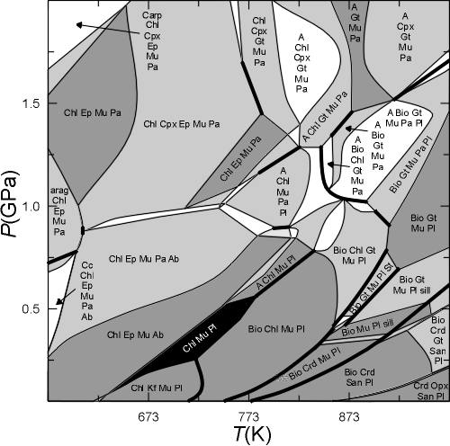
Fig 1. [Note: this figure is here because it looks nice and to provide an example of a pseudosection, the correct phase relations involve lawsonite, which was not considered in the calculation illustrated here. This diagram was constructed by "hand", as a result some phase field boundaries are incorrectly interpreted as univariant, use of the current version of PSVDRAW eliminates such errors. Stay tuned for the re-drafted figure]. Stable mineralogy for Shaw's (1956) average (sub-aluminous) metapelite composition in for a system that is open with respect to a C-O-H fluid formed by equilibration of water with graphite (Connolly, 1995). The extremely water-rich (reduced) composition of the fluid results in a restricted carbonate stability field. Quartz is stable in all phase fields of the section. The assemblages were computed using Vertex (Connolly 1990) with end-member data from Holland and Powell (1998) and solution models as detailed below. Thin solid lines indicate conditions at which minerals appear or disappear, with increasing temperature, due to a continuous reaction. Heavy solid lines locate discontinuous reactions whereby one mineral is replaced by another. Phase notation, compositions (w, x, y, and z are fractions that vary between zero and unity) and the solution models employed are: A (tremolite-tschermakite-pargasite-glaucophane amphibole, Ca2-2zNa2z+wMgxFe(1-x)Al3w+4y+4zSi8-2w-2yO22(OH)2, non-ideal, modified from Holland and Powell, 1998), Arag (aragonite, CaCO3), Ab/Kf (low Na/K feldspar, NaxKyCa1-x-yAl2-x-ySi2+x+yO8, non-ideal, Newton et al., 1980, Thompson and Waldbaum, 1969) Bio (biotite, KMg(3-y)xFe(3-y)(1-x)Al1+2ySi3-yO10(OH)2, non-ideal, Holland and Powell, 1998), Carp (carpholite, MgxFe1-xAl2Si2O6(OH)4, ideal, Holland et al., 1998), Cc (calcite, Ca1-x-yMgxFeyCO3, non-ideal, modified from Annovitz and Essene, 1987), aChl (aluminous chlorite, Mg(5-y)xFe(5-y)(1-x)Al4+2ySi3-yO10(OH)8, non-ideal, Holland et al., 1998), Crd (cordierite, Mg2xFe2-2xAl4O18(H2O)y, ideal, Holland and Powell, 1998), Cpx (low and high clinopyroxene, Na1-yCayMgxy(1-z)Fe(1-x)y(1-z)Aly+2zSi2-zO6, modified from Gasparik, 1985, Ep (epidote, Ca2Al3-x FexSi3O12(OH), non-ideal, Holland and Powell, 1998), Gt (garnet, Fe3xCa3yMg3(1-x-y)Al2Si3O12, non-ideal, Holland and Powell, 1998), Opx (Mg2xFe2-2xSi2O6, non-ideal, Holland and Powell, 1998), San (sanidine, KxNa1-xAlSi3O8, Thompson and Waldbaum, 1969), Mu/Pa (muscovite/paragonite, KxNa1-xMgyFezAl3-2(y+z)Si3+y+zO10(OH)2, non-ideal, modified from Chatterjee and Froese, 1975 and Holland and Powell, 1998), Pl (plagioclase, NaxCa1-xAl2-xSi2+xO8, Newton et al., 1980), q (quartz, SiO2), sill (sillimanite, Al2SiO5), and St (staurolite, Mg4xFe4-4xAl18Si7.5O48H4, non-deal, Holland and Powell, 1998).
The calculation outlined here is for a pelitic bulk composition in the system Na2O-MgO-Al2O3-SiO2-K2O-CaO-FeO-C-O-H as a function of pressure and temperature. Two limiting models can be applied in Perple_X to account for the behavior of volatile components (e.g., H2O, CO2 and O2). In the closed system model, the amount of the volatile components is constrained by mass balance. In most metamorphic mixed-volatile systems, this type of calculation is unrealistic because fluid flow can be expected to modify the relative proportions of the volatile components within the system. The alternative model is that of an open system. In the open system model, it is assumed that the system is saturated by a mobile fluid phase that determines the chemical potentials of the volatile components. The limitation of such a model is that, in general, the fluid composition is a function of the rate of fluid flow from external sources and the rate at which the different components are produced by devolatilization from within the system (i.e., a reactive transport problem). However, if the external fluid fluxes are large, then they may overwhelm the chemical effect of devolatilization and such a model may be appropriate.
The open system model is employed here, with the assumption that the system is in equilibrium with a fluid that is formed by the equilibration of water with excess graphite. This assumption implies that fluid speciation and oxidation state are solely a function of fluid pressure and temperature, and has been argued to provide a reasonable model for metapelite devolatilization (Connolly & Cesare 1993, Connolly 1995; see also Chap 6 of the tutorial). Among the alternative approaches that are possible in Perple_X, the presence and composition of a simple binary H2O-CO2 fluid can be specified and redox state constrained by an oxygen fugacity buffer (e.g., QFM). The disadvantage of such specifications is that they are arbitrary and do not represent limiting models. Alternative BUILD scripts for this problem are:
The following script details the prompts from the program BUILD (normal font) and user responses (bold font). Explanatory comments are written in red.
c\> build
NO is the default answer to all Y/N prompts (help)
Enter name of computational option file to be created
<100 characters, left justified: (help)
in12.dat
Enter thermodynamic data file name (e.g. hp94ver.dat), left justified: (help)
hp98ver.dat
The first major block of prompts from BUILD determine the manner in which the chemical components defined within the thermodynamic data file are to be used. VERTEX permits components to be treated in four different ways: saturated phase components are components whose chemical potentials are determined by the assumed stability of a phase, most commonly a fluid, containing these components; saturated components are components whose chemical potentials are determined by the assumed stability of a pure phase(s) and or solutions containing only the saturated-phase and saturated components; mobile components are components whose chemical potentials are defined explicitly; and thermodynamic components are components whose chemical potentials are the dependent variables of a phase diagram calculation. Phase diagram calculations require the specification of at least one thermodynamic component.
The current data base components are:
NA2O MGO AL2O3 SIO2 K2O CAO TIO2 MNO FEO O2 H2O CO2
Transform them (Y/N)?
This option would permit the user to redefine the data base components, e.g., to create Fe2O3 from the components FeO and O2.
n
Calculations with a saturated phase (Y/N)?
The phase is: FLUID
Its compositional variable is: Y(CO2), X(O), etc.
y
Select the independent saturated phase components:
H2O CO2
Enter names, left justified, 1 per line, [cr] to finish:
For C-O-H fluids it is only necessary to select volatile species present in the solids of interest. If the species listed here are H2O and CO2, then to constrain O2 chemical potential to be consistent with C-O-H fluid speciation treat O2 as a saturated component. Refer to the Perple_X Tutorial for details.
H2O
CO2
Calculations with saturated components (Y/N)?
y
In principal there is no need to introduce saturated components for this calculation, however it is convenient for two reasons:
O2: Perple_X can treat graphite saturated fluids in two ways: in terms of H2O-CO2-O2 or in terms of H2 and O2. The latter is more natural, but unfamiliar to most petrologists, thus the former technique is employed here. This technique requires that the system is "saturated" in the O2 component (See Tutorial Chap 6).
SiO2: For a pelitic composition it is probable that the system will always have quartz or a silica polymorph as a stable phase, by specifying that SiO2 is present in excess the program will run faster and generate simpler output. The disadvantage of this trick is that Perple_X will not explicitly show the silica polymorph reactions (although these are accounted for implicitly in the calculation).
**warning ver015** if you select > 1 saturated component, then the order you enter the components determines the saturation heirarchy and may effect your results (see Connolly 1990).
See also Tutorial Chap 3 for discussion of saturation hierarchies. In this case the hierarchy has no thermodynamic significance, but SIO2 is entered first so that its amount can be specified later.
Select < 6 saturated components from the set:
NA2O MGO AL2O3 SIO2 K2O CAO TIO2 MNO FEO O2
Enter names, left justified, 1 per line, [cr] to finish:
SIO2
O2
Use chemical potentials, activities or fugacities as independent variables (Y/N)? (help)
n
Select thermodynamic components from the set: (help)
NA2O MGO AL2O3 K2O CAO TIO2 MNO FEO
Enter names, left justified, 1 per line, [cr] to finish:
NA2O
MGO
AL2O3
K2O
CAO
FEO
Select fluid equation of state:
0 - X(CO2) Modified Redlich-Kwong (MRK/DeSantis/Holloway)
1 - X(CO2) Kerrick & Jacobs 1981 (HSMRK)
2 - X(CO2) Hybrid MRK/HSMRK
3 - X(CO2) Saxena & Fei 1987 pseudo-virial expansion
4 - Bottinga & Richet 1981 (CO2 RK)
5 - X(CO2) Holland & Powell 1991, 1998 (CORK)
6 - X(CO2) Hybrid Haar et al 1979/CORK (TRKMRK)
7 - f(O2/CO2)-f(S2) Graphite buffered COHS MRK fluid
8 - f(O2/CO2)-f(S2) Graphite buffered COHS hybrid-EoS fludi
9 - Max X(H2O) GCOH fluid Cesare & Connolly 1993
10 - X(O) GCOH-fluid hybrid-EoS Connolly & Cesare 1993
11 - X(O) GCOH-fluid MRK Connolly & Cesare 1993
12 - X(O)-f(S2) GCOHS-fluid hybrid-EoS Connolly & Cesare 19
13 - X(H2) H2-H2O hybrid-EoS
14 - EoS Birch & Feeblebop (1993)
15 - X(H2) low T H2-H2O hybrid-EoS
16 - X(O) H-O HSMRK/MRK hybrid-EoS
17 - X(O) H-O-S HSMRK/MRK hybrid-EoS
18 - X(CO2) Delany/HSMRK/MRK hybrid-EoS, for P 10 kb
19 - X(O)-X(S) COHS hybrid-EoS Connolly & Cesare 1993
20 - X(O)-X(C) COHS hybrid-EoS Connolly & Cesare 1993
21 - X(CO2) Halbach & Chatterjee 1982, P 10 kb, hybrid-Eo
22 - X(CO2) DHCORK, hybrid-Eos
The equation of state must be for graphite-saturated fluids as a function of the compositional variable X(O) for the fluid, i.e., choices 9-12. A disadvantage of employing this type of equation of state is that it becomes numerically unstable at low temperature conditions because the concentrations of some species may become vanishingly small.
This choice is computationally expensive, to save time choose equation of state 5 (CORK); specify only one saturated phase component(i.e., H2O), omit O2 as a saturated component, and enter 1.0 when prompted for the value of X(CO2). This configuration would imply a model with no possible redox or decarbonation processes, saturation with respect to a mobile water phase, and conservation of all other components. The section obtained is almost identical except that in the graphite saturated model epidote and carbonate are stable phases and there is a depression of the conditions for equilibrium dehydration.
10
Compute f(H2) & f(O2) as the dependent fugacities (do not unless you project through carbon) (Y/N)? (help)
The answer to this question would be yes if the user had elected to describe the fluid with components H2 and O2. However, in this case the user chooses to describe the fluid in terms of H2O, CO2, and O2 (Tutorial Chap 6)
n
Reduce graphite activity (Y/N)?
n
The second major block of prompts defines the explicit variables to be used for the phase diagram calculation.
The data base has P(bars) and T(K) as default independent potentials. Make one dependent on the other, e.g., as along a geothermal gradient (y/n)? (help)
This option would permit the user to do calulations in which one variable is used to define both the temperature and pressure of the system.
n
Specify computational mode: (help)
1 - Unconstrained minimization [default]
2 - Constrained minimization on a grid
3 - Output pseudocompound data
Unconstrained optimization should be used for the calculation of composition, mixed variable, and Schreinemakers diagrams, it may also be used for the calculation of phase diagram sections for a fixed bulk composition. Gridded minimization can be used to construct phase diagram sections for both fixed and variable bulk composition. Gridded minimization is preferable for the recovery of phase and bulk properties.
Unconstrained minimization is the original Perple_X strategy, in this mode the compositions of the thermodynamic components are normally unconstrained, in which case the compositions are implicit variables, but they may also be fixed (as in the calculation of a pseudosection for a system with a specified bulk composition). In contrast, in constrained minimization the compositions of the thermodynamic components must be specified. An advantage of constrained minimization is that it permits calculations as an explicit function of bulk composition. See the seismic velocity tutorial for an illustration of a pseudosection calculation with gridded minimization and the gridded minimization pros and cons page for additional discussion of merits and details.
Both computational modes can be used for pseudosections. In unconstrained minimization mode, the pseudosection is defined by a continuous mesh of polygons that exactly define phase stabilities. In constrained minimization mode VERTEX computes stable phase assemblages on a regular grid defined by the section variables, the phase relations for the section are then approximated by assuming that the phase assemblage at a grid point represents the phase assemblage in the area immediately around the grid point. Exactness is essentially the only advantage of the former method which is considerably more complex and may be complicated by errors that lead to holes in the polygonal mesh or other problems. The advantages of mode 2 are that it is simple, fast, and robust. The disadvantage of mode 2 is that the postscript plots generated for this mode can be very large, and that in this mode VERTEX does not explicitly identify univariant phase fields, i.e., univariant phase fields are not distinguished from high variance phase field boundaries. The plot output and user dialog for this calculation with mode 2 can be viewed in the Perple_X examples.
Mode 1 is selected here for purposes of illustration. The prompts and the subsequent analysis for Mode 2 is virtually identical, except that for mode 2 it is not necessary to use the programs POLYGON and WERAMI.
1Specify number of independent potential variables: 0 - Composition diagram [default] 1 - Mixed-variable diagram 2 - Pseudosections and Schreinemakers-type diagrams
In unconstrained minimization, only thermodynamic potentials (pressure, temperature) or directly related properties such as the composition of a saturated phase can be chosen as explicit variables. A diagram with no explicit potential variables is a composition diagram, any other diagram is technically a mixed-variable diagrams (potentials and compositions); however within Perple_X, diagrams with only one explicit independent potential variable are designated mixed-variable diagrams, whereas as diagrams with two explicit independent potential variables are designated as Schreinemakers-type diagrams if the thermodynamic components are unconstrained and as Pseudosections if the amounts of the thermodynamic components are specified.
2

Select x-axis variable:
1 - P(bars)
2 - T(K)
3 - X(O)
2

Enter minimum and maximum values, respectively, for: T(K)
The lower limit is chosen as 573 because the fluid equation of state fails at lower temperatures. The upper limit is chosen as 973 K to avoid conditions far above the wet granite solidus.
As outlined, this calculation will require roughly 10 minutes on a 200 MHz PC amd generate ca 1 Mb plot files, a substantial reduction in time and/or memory requirements can be achieved by using a narrower P-T window than specified below.
573 973
Select y-axis variable:
2 - P(bars)
3 - X(O)
2
Enter minimum and maximum values, respectively, for: P(bars)
The lower pressure limit arises from necessity, i.e., the speciation algorithm for C-O-H fluids may be unreliable at lower pressure.
Fluid produced by the equilibration of graphite with water must have a composition of X(O) = 1/3 = n(O)/{n(O)+n(H)}. The last digit is rounded up to shift the composition slightly to the oxidized side of the C-H2O join.
0.3333333333333333333334
Constrain bulk composition (as in pseudosections, y/n)?
y
Answering no above would lead to the calculation of a Schreinemakers-type phase diagram projection.
The next prompts define the components to be constrained. Answering no at any point will complete the set of constraints. The prompts are for thermodynamic components, followed by saturated components, in the order entered above. E.g., to constrain Fe:Mg enter FEO and MGO as the first two thermodynamic components, and specify the amounts of both.
The example mentioned above would be an under-constrained pseudosection, in that the number of constrained components would be less than the number of thermodynamic components. In such a section there may be than more than one phase assemblage possible in any given condition defined by the sections variables. Such sections are useful for certain purposes but cannot be analyzed by POLYGON, which requires fully constrained pseudosections. Constrained minimization mode is generally preferable for the construction of phase diagram sections as a functiion of composition.
A fully constrained pseudosection is a section in which the number of constrained components is equal to, or greater than the number of thermodynamic components. In a fully constrained section there is only one phase assemblage possible at any condition within the section.
Constrain component NA2O (Y/N)?
y
Constrain component MGO (Y/N)?
y
Constrain component AL2O3 (Y/N)?
y
Constrain component K2O (Y/N)?
y
Constrain component CAO (Y/N)?
y
Constrain component FEO (Y/N)?
y
Constrain component SIO2 (Y/N)?
Here the user specifies an over constrained system in that the amount of a saturated component is also specified. There is a potential danger in specifying the amount of a saturated component, in that the user may specify a smaller proportion of the component than is necessary for saturation. VERTEX tests the validity of such constraints and indicates when the constraints are invalid in the print file; however, the program will continue to execute regardless of the validity of the constraint.
y
Constrain component O2 (Y/N)?
If no constraint is specified for a saturated component, then the amount of this component necessary to saturate the phases of the system is computed by Perple_X at every possible condition of the system.
n
Specify constraints by weight (Y/N)?
n
Enter molar amounts of the components:
NA2O MGO AL2O3 K2O CAO FEO SIO2
for the bulk composition of interest:
Perple_X requires the amounts of the components, the units used and total value of the components have no fundamental importance, but define the molar unit for the system. For numerical reasons the molar quantities specified here should not differ by many orders of magnitude from those typical of the phases in the thermodynamic database. Rational molar amounts (1/2, 1, 0, etc.) should be avoided because this is likely to lead a situation in which the composition lies on a tie-line, in such cases there is no unique solution to the phase equilibrium problem.
The next block of prompts define the output required by the user.
Do you want a print file (Y/N)?
y
Enter the print file name, < 100 characters, left justified [default = pr]:
print12
Long print file format (Y/N)?
n
Print pseudodivariant assemblage data (y/n)?
n
Write full reaction equations (Y/N)?
n
Suppress console status messages (Y/N)?
n
Print dependent potentials for chemographies (Y/N)?
Answer no if you do not know what this means.
n
Enter the plot file name, < 100 characters, left justified [default = pl]:
plot12Specify efficiency level [1-5, default is 3]:
1 - gives lowest efficiency, highest reliability
5 - gives highest efficiency, lowest reliability
High values increase probability that a curve may be partially determined or skipped.
This prompt tends to unnerve users, the value specified can result in a significant savings of both time and space, but generally has no effect on computational results. Since the errors in pseudosections calculated by VERTEX are obvious (holes), there is no reason to worry about this parameter.
3
The final block of prompts from BUILD define the possible phases for the calculation, the following warnings identify endmember phases or species in the thermodynamic data base that cannot be defined by a positive linear combination of the selected components (although CO, CH4 and H2 are species in the saturated fluid, the rejection of these species here has no effect on the speciation calculations, which are done by internal routines).
**warning ver013** phase iron has null or negative composition and will be
rejected from the composition space.
**warning ver013** phase gph has null or negative composition and will be
rejected from the composition space.
**warning ver013** phase diam has null or negative composition and will be
rejected from the composition space.
**warning ver013** phase CO has null or negative composition and will be
rejected from the composition space.
**warning ver013** phase CH4 has null or negative composition and will be
rejected from the composition space.
**warning ver013** phase H2 has null or negative composition and will be
rejected from the composition space.
Exclude end-member phases (Y/N)?
It is simplest to begin by including all possible end-member phases. This allows the user to identify flaws in her perception of what the stable phases should be, or alternatively, problems in the thermodynamic data. Here, however, the user excludes zoisite (zo) because the epidote solution models use the monoclinic aluminous end-member and also to avoid the zoisite-clinozoisite transition, which is primarily a distraction in terms of interpreting phase equilibria.
y
Do you want to be prompted for phases (Y/N)?
n
Enter phases, left justified, one per line, [cr] to finish:
qfmzo
Do you want to treat solution phases (Y/N)?
y
Enter solution model file name (e.g. solut.dat),
left justified, < 15 characters:
solut.dat
...diagnostics omitted...
BUILD reads the solution model file and determines which solutions are consistent with the problem as specified by the user. The diagnostics (omitted here) can generally be ignored. They are useful if you discover that a solution you wish to include is not present in the list of solutions BUILD offers.
Select phases from the following list, enter one per line,
left justified, [cr] to finish
aChl T Bio St Ctd Carp
Crd hCrd Sud(Livi) Sud Cumm Gl
Tr TrTs trtspg TrTsPg trhbgl TrHbGl
feldspar Pl(h) Pl AnPl AbPl Ab(h)
Ab Kf(h) Kf San GCOHF H2OM
MaPa K-Phen KN-Phen MuPa PaCel MuCel
Pa Mu CzEpPs EpCz E(HP) E
HeDi(HP) DiCats Cpx(l) Cpx(h) O(HP) O
Do(HP) M(HP) Cc(AE) Sp(JR) Sp(GS) Sp(HP)
Sp Neph(FB) GrAd(EW) GrAd GrPyAl(G) GtD
Gt(HP) GrPyAl(B) Chl TrEdGl sChl ftr-fparg
trpargglc trgltsch GlTrTs
The "art" of using Perple_X is in the choice of solution models, to do this properly there is no alternative to actually reading the comments in the solution model file to discover the purpose of a particular model. For phases that exhibit immicibilty there are frequently two or more "solutions" that represent different compositional ranges of the same true phase, e.g., KN-Phen, MuCel and PaCel all represent phengitic K-Na mica. The reason for this is that in pseudosections Perple_X usually does not test whether coexisting pseudocompounds of the same solution are separated by a miscibility gap. Thus if a single model is used to represent the entire range of mica (i.e., KN-Phen), Perple_X will interpret coexisting paragonitic and muscovitic micas as being a single phase (See Tutorial Chapters 4 and 5 or Connolly 1990, Connolly & Kerrick 1987, Connolly & Trommsdorff 1991).
Two details of relevance here are the choice of the chlorite and glaucophane models. The three models listed here sChl, aChl and Chl are variations of the Baker et al. (1998, EJM) model, where Chl is the complete model, and aChl and sChl are for chlorites, respectively, more and less aluminous than the clinochlore-daphnite join. Both aChl and sChl are approximations that neglect the concentrations of the siliceous chlorite species in aluminous chlorites, and vice versa, an approximation that, in my experience, appears adequate for pelitic compositions. With regard to Glaucophane-bearing amphibole the real choice is bewteen Gl and GlTrTs, Gl is simply Fe-Mg exchange for the glaucophane endmember composition, whereas GlTrTs is a model that acounts additionally for A-site Ca-Na and Tschermaks exchanges. Although it might be expected that the GlTrTs model is more realistic, my suspicion is that it leads to an excessive amphibole stability field and hence I have used the Gl model here. However, for the record, note that the pseudosections presented in the Kerrick & Connolly (2001a,b) and Connolly & Petrini (2002) papers were calculated with the GlTrTs model.
aChl
Bio
St
Carp
hCrd
Gl
TrTsPg
AbPl
Kf
San
PaCel
MuCel
EpCz
E(HP)
Gt(HP)
Cpx(l)
Enter a title for your calculation:
Test Problem 12
The user dialog with the program VERTEX consists of entering the name of the computational option file created by BUILD (in12.dat) and, optionally, for phase diagram sections, the stable assemblage at the initial conditions. VERTEX writes diagnostics to the users console and completes the calculation. The only difference in this dialog to that for other types of calculations with VERTEX is that VERTEX creates two additional files. The names of these files are formed adding the prefixes "b" and "p" to the plot file name specified by the user in BUILD, i.e., in this example the user has specified the plot file name "plot12" while running BUILD and VERTEX will therefore create three files plot12, bplot12 and pplot12. It is only necessary to be aware of these files if you wish to store or analyze results in a different directory than the working directory for VERTEX.
c\> vertex
Enter computational option file name (i.e. the file created
with BUILD), left justified:
in12.dat
Reading thermodynamic data from file: hp98ver.dat
Writing print output to file: pr12
Writing plot output to file: plot12
Writing bulk composition plot output to file: bplot12
Initializing polygon output file: pplot12
Reading solution models from file: solut.dat
...
The console output (omitted here) consists of information and warnings on the solution models to be used in the calculation. These messages inform the user as to which solution models in the solution model file are compatible with the problem definition, i.e., that the solution end-members are possible phases for the calculation. If only a subset of the solution model end-members are present, the messages indicate how the model is to be reformulated in terms of this subset. If you do not get the solution models you requested, or if you get different solution compositions than you expect, these messages may be helpful.
The remaining console output (omitted here) consists of diagnostics and progress information. The significance of any warnings generated by VERTEX is most easily assessed by viewing the computational results graphically.
The print file (print12) created for pseudosection calculations is in large part similar to that created for other types of calculations (See Tutorial Chaps 2-4, & 9). For a complex calculation such as considered here, the print file may be extremely large, but it is nonetheless wise to scan the header and other major components of the file to verify that the computation was in fact set up in the way intended. In contrast to other types of calculations, for fully constrained bulk composition computations VERTEX also outputs data describing the bulk chemistry, modes, and physical properties in all the high variance fields of the calculation, e.g.:
(1) Stable phases at:
T(K) = 573.000
P(bars) = 500.000
X(O) = 0.333333
Molar Phase Compositions:
mol % wt % vol %
NA2O MGO AL2O3 K2O CAO
FEO SIO2 O2 H2O
CO2
MuCel(020)
10.46 27.73 26.33
0.01 0.05 1.27 0.49 0.00
0.20 3.28 0.00 1.01 0.00
MuCel(020)
0.65 1.73 1.64
0.01 0.05 1.22 0.49 0.00
0.25 3.34 0.00 1.01 0.00
aChl(cl44-99)
1.16 4.82 4.32
0.00 2.25 1.00 0.00 0.00
2.75 3.00 0.00 4.00 0.00
aChl(cl40-99)
2.82 11.93 10.56
0.00 2.00 1.00 0.00 0.00
3.00 3.00 0.00 4.00 0.00
ab
9.42 16.05 16.67
0.50 0.00 0.50 0.00 0.00
0.00 3.00 0.00 0.00 0.00
wrk
3.39 9.58 11.36
0.00 0.00 1.00 0.00 1.00
0.00 4.00 0.00 2.00 0.00
q
72.10 28.15 29.12
0.00 0.00 0.00 0.00 0.00
0.00 1.00 0.00 0.00 0.00
Molar Properties:
N(g)
H(J) V(J/bar) Cp(J/K)
Alpha(1/K) Beta(1/bar)
MuCel(020)
407.96 -0.53518E+07 14.361
452.49 0.34467E-04 0.20886E-05
MuCel(020)
410.50 -0.53417E+07 14.406
453.87 0.34467E-04 0.20834E-05
aChl(cl44-99)
642.58 -0.69754E+07 21.323
753.21 0.22879E-04 0.22000E-05
aChl(cl40-99)
650.46 -0.68866E+07 21.336
754.43 0.22879E-04 0.22001E-05
ab
262.23 -0.35750E+07 10.097
283.02 0.32557E-04 0.17930E-05
wrk
434.41 -0.59720E+07 19.094
514.66 0.13734E-04 0.10408E-05
q
60.09 -0.82766E+06 2.3040
63.497 0.38529E-04 0.19789E-05
System
10018.89 -0.13057E+09 371.39
11079. 0.31252E-04 0.19049E-05
mol mol %
wt %
NA2O 3.16
1.88 1.95
MGO 5.73
3.40 2.31
AL2O3 17.00
10.09 17.30
K2O 3.56
2.11 3.35
CAO 2.21
1.31 1.24
FEO 9.05
5.37 6.49
SIO2 105.70
62.73 63.40
O2 0.00
0.00 0.00
H2O 22.09
13.11 3.97
CO2 0.00
0.00 0.00
Density(kg/m3) =
2697.7
Specific Enthlpy (J/m3) = -.351580E+11
Specific Heat Capacity (J/K/m3) = 0.298325E+07
Variance (c-p+2) = 4
This output is largely self-explanatory for users familiar with the Perple_X pseudocompound approximation (e.g., Tutorial Chap 4, 9), however a few clarifications may be helpful:
V = Vref (1 + a (T-Tref) - b (P-Pref))
where Vref, Pref and Tref are the molar volume, pressure and temperature specified in the output (e.g., 573 K and 500 bar in the above case) and a and b are the isothermal compressibility and the isobaric expansivity.
What does POLYGON do? The pseudounivariant fields that bound the stability of any given pseudodivariant assemblage define a curvilinear polygonal field within a pseudosection. The program POLYGON assembles these polygons from VERTEX's output (the "plot" file plot12, and the assemblage plot file bplot12 named by adding the prefix "b" to the plot file name specified by the user in BUILD), which consists of stable pseudounivariant curve segments. In essence, POLYGON creates a digital polygonalized map of a pseudosection.
Why use POLYGON? POLYGON constructs the 2-dimensional curvilinear polygonal fields corresponding to each pseudodivariant assemblage. Since the physical properties of the assemblage in these fields are known from VERTEX, the polygonal fields can be shaded in graphics programs to permit visualization of the properties or the assemblages as a function of the pseudosection variables. POLYGON is therefore useful in the graphical analysis of a pseudosection with PSVDRAW. The polygonalized map of a pseudosection permits rapid digital recovery of the physicochemical properties of the rock system in question. Such maps are useful for thermal, mechanical and chemical computational models of petrological systems. The map can be manipulated graphically (PSVDRAW) or interpreted directly (WERAMI).
The dialog with POLYGON may involve modification of the default memory allocation defined within the program, but otherwise consists only of entering the name of the plot file created by VERTEX (plot12). POLYGON writes diagnostics to the users console and completes the "polygon" plot file initialized by VERTEX (this file is named by adding the prefix "p" to the plot file name specified by the user in BUILD, i.e., in this example the "polygon" plot file is named pplot12).
c\> polygon
Change default memory allocation (y/n)?
y
Unlike the other Perple_X programs, Polygon is written in FORTRAN90 and uses dynamic memory allocation. To avoid making the program so large that it becomes inefficient, the default dimensioning is set to moderate values. For problems such as the example here, this dimensioning is inadequate and must be changed. If polygon is run with inadequate dimensioning the program writes a diagnostic indicating the parameter that should be changed.
Change the maximum number of stable assemblages (noass=1000, y/n)?
y
enter new value:
The correct value to be entered here can be determined by trial and error or by reading the maximum number of assemblages from the print file (print12) or the assemblage plot file (bplot12).
2500
Change the maximum number of curve segments (maxseg=5000, y/n)?
This parameter is greater than or equal to the number of pseudounivariant equilibria listed in the print file.
n
Change the maximum number of coordinates on any curve segment (maxncoor=200, y/n)?
y
enter new value:
400
Change the maximum number of curve segments that bound any pseudodivariant field (maxseg_per_pol=15, y/n)?
n
Enter plot file name:
plot12
Constructing polygons
Polygon bounding assemblage 279 is incomplete
Polygon bounding assemblage 316 is incomplete
These diagnositics indicate that the polygonal field of the indicated pseudodivariant assemblage is not completely defined. Currently incomplete fields are plotted by PSVDRAW (and indicated with a solid symbol, to distinguish them from normal fields), but are considered to define regions of missing data by WERAMI. Problems leading to an incomplete field are related to numerical tolerances and may arise in either VERTEX or POLYGON.
...output abridged...
preparing output
writing output
We have not verified that the code is as
transportable as other components of Perple_X.
Katja Petrini tested and developed POLYGON under WINDOWS/NT. The program does
compile and run correctly under IRIX/SGI. POLYGON has large default memory (or
virtual memory) requirements (ca 20 Mbyte). This may require that WINDOWS users
increase the size of the system paging file. If POLYGON runs out of memory, the
program may crash with misleading system diagnostic messages or in some
instances with no diagnostics at all. In some cases POLYGON may terminate with a
message indicating that the allocation specified by a parameter must be
increased. If this recurs after the parameter has been increased beyond
reasonable limits it is likely that the problem is related to WINDOWS memory
management problems and additional memory should be made available by
terminating other applications or increasing the virtual memory for the system.
The current version of POLYGON has a bug that sometimes causes it to
misinterpret polygons at the corners of the diagram with the error results
in a polygon that fills the upper or lower diagonal of the diagram and
overprints the correct phase relations. A symptom of this problem is that the
shading of the affected phase fields (using the default plot mode of PSVDRAW)
does not vary across phase field boundaries. When this error occurs the diagram
can be corrected by deleting the erroneous polygon with a graphical editor.
(Alternatively use VERTEX's second computational mode to
eliminate the necessity of POLYGON).
What does WERAMI do? Once a pseudosection has been polygonalized with POLYGON, WERAMI permits the user to extract information from the section at a point, throughout a region, or along a line or curve. The latter two options generate output that can be plotted with programs PSCONTOR or PSPTS. The dialog and output for each of these modes is detailed below:
In this mode, the user specifies a set of physical conditions and WERAMI determines the stable phase assemblage, and its properties, from the output created by VERTEX and POLYGON.
c\> werami
Enter the VERTEX plot file name:
plot12
The input file for WERAMI is the plot file created by VERTEX, not the plot file written by POLYGON (pplot12).
Select operational mode:
1 - compute properties at specified conditions
2 - create a property grid (plot with pscontor)
3 - compute properties along a curve or line (plot with pspts)
4 - as in 3, but input from file.
5 - compute properties of a specified (by index) assemblage
1
Console output will be echoed in file: rplot12
The console echo provides a useful summary, but is not used by any other Perple_X programs. The echo file name is formed by concatenating the plot file name (plot12) with the character "r".
Enter T(K) and P(bar) (zeroes to quit):
574 501
Once the users specifies conditions, WERAMI scans the polygonal fields defined by POLYGON to determine if the conditions lie within the stability field of a pseudodivariant assemblage identified by VERTEX. The algorithm strictly locates points within the polygonal fields, therefore it is important to avoid specifiying conditions that lie on the edge of the pseudosections coordinate frame, e.g., specifying 573 K/500 bar here would cause WERAMI to return a "Missing Data" diagnostic. This diagnostic message may also be returned if a point lies within a gap in the polygonal mesh defined by VERTEX and POLYGON.
(1) Stable phases at:
T(K) = 574.000
P(bar) = 501.000
X(O) = 0.333333
Molar Phase Compositions:
mol % wt % vol %*
NA2O MGO AL2O3 K2O
CAO FEO SIO2 O2
H2O CO2
MuCel(020)
10.46 27.73 26.33 0.01
0.05 1.27 0.49 0.00 0.20
3.28 0.00 1.01 0.00
MuCel(020)
0.65 1.73 1.64
0.01 0.05 1.22 0.49 0.00
0.25 3.34 0.00 1.01 0.00
aChl(cl44-99)
1.16 4.82 4.32
0.00 2.25 1.00 0.00 0.00
2.75 3.00 0.00 4.00 0.00
aChl(cl40-99)
2.82 11.93 10.56 0.00
2.00 1.00 0.00 0.00 3.00
3.00 0.00 4.00 0.00
ab
9.42 16.05 16.67
0.50 0.00 0.50 0.00 0.00
0.00 3.00 0.00 0.00 0.00
wrk
3.39 9.58 11.36
0.00 0.00 1.00 0.00 1.00
0.00 4.00 0.00 2.00 0.00
q
72.10 28.15 29.12
0.00 0.00 0.00 0.00 0.00
0.00 1.00 0.00 0.00 0.00
Molar Properties*:
N(g) H(J)
V(J/bar) Cp(J/K)
Alpha(1/K) Beta(1/bar)
MuCel(020)
407.96 -0.53518E+07 14.361 452.49
0.34467E-04 0.20886E-05
MuCel(020)
410.50 -0.53417E+07 14.406
453.87 0.34467E-04 0.20834E-05
aChl(cl44-99)
642.58 -0.69754E+07 21.323
753.21 0.22879E-04 0.22000E-05
aChl(cl40-99)
650.46 -0.68866E+07 21.336
754.43 0.22878E-04 0.22001E-05
ab
262.23 -0.35750E+07 10.097
283.02 0.32557E-04 0.17930E-05
wrk
434.41 -0.59720E+07 19.094
514.66 0.13734E-04 0.10408E-05
q
60.09 -0.82766E+06 2.3040
63.497 0.38529E-04 0.19789E-05
System
10018.90 -0.13057E+09 371.39
11080. 0.31252E-04 0.19049E-05
mol mol %
wt %
NA2O 3.16
1.88 1.96
MGO 5.73
3.40 2.30
AL2O3 17.00
10.09 17.31
K2O 3.56
2.11 3.35
CAO 2.21
1.31 1.24
FEO 9.05
5.37 6.49
SIO2 105.70
62.73 63.41
O2 0.00
0.00 0.00
H2O 22.09
13.11 3.97
CO2 0.00
0.00 0.00
Density (kg/m3)** = 2697.6
Specific Enthlpy (J/m3)** = -.351539E+11
Specific Heat Capacity (J/K/m3) = 0.298317E+07
Variance (c-p+2) = 4
*Computed at
reference condition (P(bar) = 500, T(K) = 573).
**Computed from linearized equation of state
relative to the reference condition.
Enter T(K) and P(bar) (zeroes to quit):
0 0
The output from WERAMI in mode 1, is essentially identical to the print file information output by VERTEX, with the exception that physical properties are computed by VERTEX using the complete equation of state for the physical entity in question. This computation is made at one condition (the " reference condition") within the stability field of the pseudodivariant assemblage. Properties reported by WERAMI are (as indicated) either the properties determined at the reference condition by VERTEX, or properties computed by WERAMI by linear extrapolation from the reference condition. The linearized forms used by WERAMI are:
V
= Vref (1 + a (T-Tref) -
b (P-Pref))
H = Href +
Cp (T-Tref) + V (P-Pref)
where Href, Cp, Vref, a, b, Pref and Tref are properties at the reference condition.
The simplest method of representing the information within a polygonalized pseudosection is with false color plots generated with PSVDRAW. However, for many purposes, it may be useful to present information on a regularly spaced grid. Such grids can be created using the second mode of WERAMI. The Perple_X program PSCONTOR can be used to visualize such data. We demonstrate these capabilities here with an example in which we contour the composition of plagioclase (and garnet) for thermobarometric purposes:
c\>werami
Enter plot file name:
plot12
The input file for WERAMI is the plot file created by VERTEX, not the plot file written by POLYGON (pplot12).
Select operational mode:
1 - compute properties at specified conditions
2 - create a property grid (plot with pscontor)
3 - compute properties along a curve or line (plot with pspts)
4 - as in 3, but input from file.
5 - compute properties of a specified (by index) assemblage
2
Select a property:
1 - Bulk specific enthalpy (J/m3)
2 - Bulk density (kg/m3)
3 - Bulk specific Heat capacity (J/K/m3)
4 - Bulk expansivity (1/K, for volume)
5 - Bulk compressibility (1/bar, for volume)
6 - Weight percent of a component
7 - Mode (Vol %) of a compound or solution
8 - Composition of a solution
Bulk properties computed for the solid assemblage.
For fluid + solid bulk properties change flag IFLU.
8
Enter solution or compound name (left justified):
AbPl
The compositional variable of interest for AbPl(plagioclase) is XCa, but this variable must be defined for WERAMI:
Compositions are defined as a ratio of the form:
w(j)*n(j) / Sum {w(i)*n(i), i = 1, c}
n(j) = number of moles of component j
w(j) = weighting factor of component j (usually 1)
The components defined for VERTEX are not necessarily ideal for the description of a particular phase as illustrated here. The user can partially correct for this limitation by specifying stoichiometric weighting factors (w(j), above).
Component index and weighting factor for the
compositions numerator?
1 - NA2O
2 - MGO
3 - AL2O3
4 - K2O
5 - CAO
6 - FEO
7 - SIO2
8 - O2
9 - H2O
10 - CO2
5 1
This implies that the numerator of the composition is the number of moles of CaO (the fifth component, with a weighting of 1).
How many components in the denominator of the composition?
2
Users can enter a zero here to obtain a plot of the "numerator" specified in response to the previous prompt.
Component indices and weighting factors for the
compositions denominator?
1 - NA2O
2 - MGO
3 - AL2O3
4 - K2O
5 - CAO
6 - FEO
7 - SIO2
8 - O2
9 - H2O
10 - CO2
5 1 1 2
This implies the denominator of the composition is the number of moles of CaO plus NaO0.5, where the weighting factor of the system component Na2O (component 1) is specified as 2, to convert the system component Na2O to the phase component NaO0.5.
The compositional variable is: 1.0 CAO / Sum 1.0 CAO 2.0 NA2O
Happy (y/n?)
y
Change default variable range (y/n)?
n
Enter number of nodes in and x and y directions:
400 400
Contours of mineral modes and compositions are highly irregular and require high resolution grids, a 100 x 100 grid is adequate for most purposes.
Writing grid data to file: cplot12
The grid data is written to a file created by concatenating "c" with the plot file written by VERTEX.
Missing data at: 952.798 2469.71
Missing data at: 964.919 2666.68
Missing data at: 944.717 3454.56
...
The missing data diagnostics indicate that a grid point lies within a gap in the polygonal mesh defined by VERTEX and POLYGON, the value of the property of interest is set equal to zero at these points and typically appears as a "hole" if the data is visualized by contouring or false color imaging.
The "holes" in property grids can be "repaired" with
the program INTERPMATRIX, which uses linear interpolation to fill the holes in
two-dimensional property grids generated by WERAMI. In general, it is wise to
examine plots prepared without INTERPMATRIX before using this program because
large holes may cause peculiar results.
c> interpmatrix
Enter grid data file name:
cplot12
The input file here is the grid data file generated by WERAMI, not the plot file generated by VERTEX.
reading data
interpolating matrix
writing interpolated grid data to file: icplot12
The repaired grid data is named by adding the prefix "i" to the original contour plot file.
The grid data can be plotted by various commercial packages such as MatLab or Maple, alternatively (the relatively crude) Perple_X program PSCONTOR can be used to generate an interpreted PostScript plot:
c\> pscontor
Enter the contour plot file name:
cplot12
The input file here is the grid data file generated by WERAMI, not the plot file generated by VERTEX. Alternatively, had INTERPMATRIX been used to repair the grid, the repaired grid data file "ciplot12" could be entered here.
PostScript will be written to file: cplot12.ps
Reset plot limits (y/n)?
n
Modify default drafting options (y/n)?
answer yes to modify:
- picture transformation
- x-y plotting limits
- relative lengths of axes
- text label font size
- line thickness
- curve smoothing
- axes labeling and gridding
n
Contoured variable range 0.0000000E+00 0.2812280
Modify default contour interval (y/n)?
Because missing data is assigned a -1 value by WERAMI, the range indicated here can be misleading (although it is not in this specific case).
y
Enter min, max and interval for contours:
0.0 0.28 0.02
The contour plot shown below was made from PostScript file generated from the preceeding dialog. The plot has been augmented by overlaying the output of a second calculation of isopleths for the Mg-content of garnet (i.e., the pyrope-content). The plot has been modified so that areas of "missing data" are shown in black, rather than as potential wells, as in the original plots. By default PSCONTOR uses thick lines to locate the minimum and maximum contours, the contour line pattern alternates between solid and broken lines, begining with the minimum contour level which is indicated by a heavy solid line. The plot demonstrates that when the use of a pseudosections is justified, pseudosections provide an extraordinarily simple thermobarometric method.
Mineral isopleths computed with WERAMI may be highly irregular due to abrupt changes in phase composition across univariant phase fields and because of discontinuities resulting from the pseudocompound approximation. Within a given true phase field, the composition of a solution can vary because the composition of the pseudocompounds change across a pseudodivariant field boundary, or because the relative proportions of two or more pseudocompounds representing the solution change across a pseudodivariant field boundary. The second effect implies that it is possible to obtain compositional resolution that is better than implied by the spacing of the pseudocompounds in phase fields with a true variance greater than two. For example, the plagioclase pseudocompounds have been generated with a spacing of ca 4 mol % an component, but a contour spacing of 2 mol % was specified for contouring. The result is that where there is only one plagioclase pseudompound stable, the variation in plagioclase composition must occur in steps of 4 mol %, which are defined by two essentially coincident contours. These contours diverge in phase fields where two plagioclase pseudocompounds are stable, but may vary in a highly irregular fashion (e.g., the 25 mol % an contour) as a consequence of the pseudocompound approximation.
In mode 3, WERAMI can be used to compute physical properties along a line passing between two user specified endpoints. The data can be plotted using the Perple_X programs PSPTS and PSVDRAW (in conjunction with PT2CURV). We illustrate this mode by computing the water content of the pelite model rock along a geothermal gradient. Refer to earlier WERAMI dialogs for clarification of the user prompts.
c\>werami
Enter the VERTEX plot file name:
plot12
Select operational mode:
1 - compute properties at specified conditions
2 - create a property grid (plot with pscontor)
3 - compute properties along a curve or line (plot with pspts)
4 - as in 3, but input from file.
5 - compute properties of a specified (by index) assemblage
3
Select a property:
1 - Bulk specific enthalpy (J/m3)
2 - Bulk density (kg/m3)
3 - Bulk specific Heat capacity (J/K/m3)
4 - Bulk expansivity (1/K, for volume)
5 - Bulk compressibility (1/bar, for volume)
6 - Weight percent of a component
7 - Mode (Vol %) of a compound or solution
8 - Composition of a solution
Bulk properties computed for the solid assemblage.
For fluid + solid bulk properties change flag IFLU.
6
Enter a component:
1 - NA2O
2 - MGO
3 - AL2O3
4 - K2O
5 - CAO
6 - FEO
7 - SIO2
8 - O2
9 - H2O
10 - CO2
9
Writing profile to file: cplot12
The plot data (i.e., the profile) file name is the same as for mode 2 calculations, be careful not to confuse files output for different modes because the plotting programs (PSCONTOR/PSPTS/PSVDRAW) will fail with the wrong input files.
Enter endpoint 1 (T(K) -P(bar) ) coordinates:
573.1 5000
The endpoints are chosen to yield a line approximating a 20 K/km geotherm. The points must be placed within the coordinate frame of the diagram to avoid missing data.
Enter endpoint 2 (T(K) -P(bar) ) coordinates:
972.9 12000
How many points along the profile?
200
Select independent variable:
1 - T(K)
2 - P(bar)
1
The choice of independent variable is significant if the profile is made parallel to one axis of the section. The profile property is shown as a function of the independent variable, which is plotted on the x-axis.
Construct a non-linear profile (y/n)?
n
By responding yes to this prompt, the user can specify the dependent variable as a polynomial function of the independent variable, the polynomial must have the general form:
y = sum (ci*xi, i = 0..n)
where n is the order of the polynomial and ci is the coefficient of the ith order term. To save time typing it is wise to enter this data in a file (WERAMI option 4), the format of this file (named 'geotherm.dat') is described in README_WERAMI.
T(K) P(bar) Property
573.100 5000.00 3.64308
...
972.900 12000.0 1.41244
Data written to the plot file is echoed to the console.
Profile data can be plotted by commercial packages such as MatLab or Maple, alternatively (the relatively crude) Perple_X program PSPTS can be used to generate an interpreted PostScript plot.
c\>pspts
Enter the point plot file name:
cplot12
PostScript will be written to file: cplot12.ps
Modify the default plot (y/n)?
n
The plot created by PSPTS consists simply of the points output by WERAMI. If the user wishes to plot curves, the Perple_X program PT2CURV can be used to convert the point data file output by WERAMI (cplot12) to the curve format used by PSVDRAW. The curves can then be plotted with PSVDRAW.
c\>pt2curv
Input file?
cplot12
Output file?
ccplot12
c\>psvdraw
Enter the point plot file name:
ccplot12
PostScript will be written to file: cplot12.ps
Modify the default plot (y/n)?
n
Water Content Along a Geothermal Gradient of 20 K/km
PSVDRAW generates PostScript graphical output and can be used once the pseudosection has been calculated with VERTEX and, preferably, polygonalized with POLYGON. A few illustrations of the way PSVDRAW can be used more effectively are given below:
c\> psvdraw
Enter plot file name:
plot12
PostScript will be written to file: plot12.ps
This PostScript file contains the graphical output from PSVDRAW, it can be viewed in any PostScript viewing tool (e.g., Ghostscript). The graphical output can be edited in generic PostScript editors such as the X-Windows application Idraw, alternatively the PostScript may be imported into graphical editors such as Illustrator or Corel.
Modify the default plot (y/n)?
The default pseudosection plot generated by PSVDRAW shows true phase fields coded by variance and labeled by phase names, however yes is entered here to illustrate some of the options for PSVDRAW.
y
Modify default drafting options (y/n)?
answer yes to modify:
- picture transformation
- x-y plotting limits
- relative lengths of axes
- text label font size
- line thickness
- curve smoothing
- axes labeling and gridding
This question refers to cosmetic options, the user answers yes to locate the axis tic marks at rational intervals.
y
Modify x-y limits (y/n)?
n
Modify default picture transformation (y/n)?
n
Modify ratio of x to y axis length(y/n)?
n
Modify default text scaling (y/n)?
n
Use minimum width lines (y/n)?
n
Fit curves with B-splines (y/n)?
n
Restrict phase fields by variance (y/n)?
answer yes to:
- draw curves and points that do not correspond to true phase boundaries
- suppress all phase boundaries
n
This prompt is only issued for Mode 1 calculations. The default obtained by answering no here is to suppress pseudounivariant curves that separate pseudodivariant phase assemblages that represent the same true phase assemblage with different phase compositions. Such curves, which define the polygonal mesh of the pseudosection, can be shown when the compositional variations of the phases within a true phase field are of interest (as in thermobarometry, see dialog 3).
Restrict phase fields by phase identities (y/n)?
answer yes to:
- show fields that contain a specific assemblage
- show fields that do not contain specified phases
- show fields that contain any of a set of specified phases
n
This option is used in dialog 3.
Modify default equilibrium labeling (y/n)?
answer yes to:
- Show [pseudo-] univariant curve labels
- Show [pseudo-] invariant point labels
- modify/suppress [pseudo-] high variance field labels
y
The default for pseudosections is to suppress invariant and univariant field labels and to label higher variance phase fields by the phases of the field. Here the default is modified so that the range of water content in each high variance phase field will be indicated.
Show curve labels (y/n)?
n
Show point labels (y/n)?
n
Label all high variance phase fields (y/n)?
n
Indicate the range of a property in labels (y/n)?
y
Indicate the range of a property in labels (y/n)?
y
Select a property:
1 - Bulk specific enthalpy (J/m3)
2 - Bulk density (kg/m3)
3 - Bulk specific Heat capacity (J/K/m3)
4 - Bulk expansivity (1/K, for volume)
5 - Bulk compressibility (1/bar, for volume)
6 - Weight percent of a component
7 - Mode (Vol %) of a compound or solution
8 - Composition of a solution
Bulk properties computed for the solid assemblage.
For fluid + solid bulk properties change flag IFLU.
6
Enter a component:
1 - NA2O
2 - MGO
3 - AL2O3
4 - K2O
5 - CAO
6 - FEO
7 - SIO2
8 - O2
9 - H2O
10 - CO2
9
Values of properties that vary as a function of the pseudosection variables at constant phase composition (e.g., density or enthalpy) are computed at the centroid of each divariant field.
Suppress phase names (y/n)?
n
Change default phase field fill patterns (y/n)?
answer yes to:
- suppress default variance-based phase field patterns
- generate fills based on the value of a property
n
assemblage 1116 not found? 574.9960 8368.860
This diagnostic indicates that VERTEX output a pseudodivariant field (1116 in the print file print12) that is not limited by any pseudounivariant field. In this case, it reflects a computational error that arises because the equation of state used for the C-O-H fluid speciation calculation fails at low temperature and high pressure (the problem could be avoided by using a simpler model for the fluid phase, e.g., CORK).
Modify default axes (y/n)?
This prompt is only given if the user indicates that she wishes to modify the default drafting options.
y
Enter the starting value and interval for major tick marks on
the X-axis (the current values are: 573. 80.0 )
Enter the new values:
573 100
Enter the starting value and interval for major tick marks on
the Y-axis (the current values are: 500. 0.390E+04)
Enter the new values:
5000 5000
Cancel half interval tick marks (y/n)?
n
Draw tenth interval tick marks (y/n)?
n
Rescale axes text (y/n)?
n
Turn gridding on (y/n)?
n
NOTE: The results illustrated here may differ from those obtained using the current version of Perple_X due to changes in the solution model subdivision schemes specified in solut.dat. The output generated from the current Perple_X version can be viewed in the Perple_X examples directory (plot #12 and dialog #12).
The figure below is from the postscript output (plot12.ps) generated by the forgoing dialog. The labels in some fields have been deleted or moved for legibility, and quartz, which is present in all fields has been omitted from the field labels. The solution names have been simplified by editing the names written to the plot file, e.g., the solution names AbPl, TrTsPg and Cpx(l) have been changed to Pl, Hbd and Cpx. The numbers in the labels preceding the phase assemblage indicate the range of water contents that occur within the pseudodivariant phase fields of each true phase field. A circle is plotted directly to the right of each label, in cluttered diagrams this circle can be used to determine the correspondence of labels to fields. If the user uses POLYGON it is absolutely certain that the circle associated with any label lies within the appropriate field, if, however, PSVDRAW is used without first running POLYGON it is possible that the circle may be positioned outside of strongly curved phase fields. The Phase assemblages within phase fields can also be deduced from the general rule that adjacent phase fields (whereby univariant curves are counted as fields as well) always differ by exactly one phase. Gray-scale fills distinguish the variance of each field, white fill indicates divariant fields, higher variance fields are progressively darker. Technical drafting problems such as axes labeling can be repaired by modifying the default drafting options in the PSVDRAW dialog. Phase compositions (pseudocompounds) are not indicated unless the user requests the labeling of all phase fields (see Dialog 3), in the present case the diagram consists of ca 2400 pseudodivariant fields and the labeling of these fields would produce a completely illegible diagram. Some problems and details of interpretation are addressed below with reference to the points labeled in the figure.
A Numerical problems in VERTEX may lead to a situation in which the boundaries of a pseudodivariant fields are not completely determined. As a result there are white "holes" in the pseudosection. These holes can be distinguished from divariant fields because their perimeter is not completely defined by pseudounivariant curves. The "holes" at low temperature and high pressure (8 kbar) are due to the failure of the fluid speciation code at conditions where the fluid becomes essentially pure water. To avoid these it would be necessary to choose a different fluid equation of state. Holes at high temperature and pressure (e.g., 843 K and 4.4 kbar) can sometimes be avoided by increasing the computational reliability level specified in the BUILD dialog.
B In a correct pseudosection, two adjacent phase fields of the same variance can only be separated by a 1-dimensional boundary if the one dimensional boundary corresponds to a true univariant curve (normally drawn by PSVDRAW with a heavy solid line). However, because of the finite compositional resolution of the pseudocompound approximation, it is not uncommon that two fields of equal variance may be separated by a pseudounivariant boundary as at point B. In such cases the assemblage of the pseudounivariant field represents the geometrically degenerated phase field of lower variance that should separate the fields of equal variance.
C Phase field boundaries frequently have jagged boundaries Because of the finite resolution of the pseudocompound. To some extent this jaggedness can be removed by increasing the compositional resolution specified for the solutions in the solution model data file (solut.dat). However, since the pseudocompound approximation gives correct average trends, with experience it is possible to smooth the boundaries by hand to obtain a reasonable approximation of the true phase field shapes. Thus, the true phase field of Mu+Chl+Gl+Pa+Cpx+law(+q+fluid) (point C) can be expected to have the shape outlined by the red curves.
D In the present calculation two solution models were used for amphibole: glaucophane (Gl) and hornblende (Hbd, i.e., TrTsPg in solut.dat), these models give plausible results over relatively broad pressure-temperature ranges. However, the use of two solution models to represent what is probably a single natural amphibole solution leads to complications in the pressure temperature region in which the amphibole compositions are transitional between those of the Gl and Hbd (fields D1-D4). As an example consider the field D1, which VERTEX/POLYGON/PSVDRAW identify as consisting of two "true" phase fields, the divariant field Pa+Chl+Gt+Mu+Hbd+Gl(+q) and the trivariant field Pa+Chl+Gt+Mu+Gl(+q). Since both Gl and Hbd represent amphibole, it is apparent that the correct "true" variance of the field Pa+Chl+Gt+Mu+Hbd+Gl(+q) is trivariant, and that this field is simply the low pressure extension of the trivariant field Pa+Chl+Gt+Mu+Gl(+q). The "true" univariant curves that bound the lower pressure limit of D1 are likewise artifacts that describe reactions between the Gl and Hbd, and are properly interpreted as pseudounivariant curves. The interpretation of the true phase relations represented in fields D2-D4 is similar, the correct variance of these fields being four, three, and three, respectively. In the final drafted version of the pseudosection I would smooth the boundaries of the fields as in C.
E The different feldspar structural states creates a problem in the interpretation of plagioclase phase relations across the narrow phase fields that extend diagonally across the section from point E. The problem here is caused by the fact that the plagioclase solution model AbPl (Pl) is defined in terms of high albite and that there is no plagioclase model with the ordered low temperature end member ab. This low temperature end member is, however, necessary to describe the low temperature alkali feldspar (Kf) and is therefore included in the calculation (the end member flag in the solution model file has been set so that the end member ab is not specifically associated with the Kf solution, see the Program Documentation Chap 4, Read 7). Consequently, there is a transition from pure low albite to albitic plagioclase across the phase fields extending from point E. The interpretation of the transition is to some extent a matter of opinion, my personal bias would be discount the entire transition as an artifact, although, if incorporated a low plagioclase solution model would in fact produce such a transition.
This dialog illustrates the use of PSVDRAW to construct a gray-scale map of an assemblage property for a pseudosection. In this case the property is the mode of a solution (garnet). This construction provides the most honest view of properties in a polygonalized section, but in most cases contour plots generated with WERAMI are more useful for quantitative applications.
c\> psvdraw
Enter plot file name:
plot12
PostScript will be written to file: plot12.ps
Modify the default plot (y/n)?
y
Modify default drafting options (y/n)?
answer yes to modify:
- picture transformation
- x-y plotting limits
- relative lengths of axes
- text label font size
- line thickness
- curve smoothing
- axes labeling and gridding
n
Restrict phase fields by variance (y/n)?
answer yes to:
- show curves and points that do not correspond to true phase boundaries
- suppress all phase boundaries
n
Restrict phase fields by phase identities (y/n)?
answer yes to:
- show fields that contain a specific assemblage
- show fields that do not contain specified phases
- show fields that contain any of a set of specified phases
n
Modify default equilibrium labeling (y/n)?
answer yes to:
- Show [pseudo-] univariant curve labels
- Show [pseudo-] invariant point labels
- modify/suppress [pseudo-] high variance field labels
y
Show curve labels (y/n)?
n
Show point labels (y/n)?
n
Label all high variance phase fields (y/n)?
n
Indicate the range of a property in labels (y/n)?
y
Indicate the range of a property in labels (y/n)?
If the user elects to label only true phase fields he is then given the option of indicating the range of a property in the phase field label. The property need not be the same as the property used for determining the gray-scale shading. The range of the property is taken as the range of the property computed at the centroids of the pseudodivariant fields that comprise the true phase field. If the true phase field corresponds to a single pseudodivariant field then a single value is given.
y
Select a property:
1 - Density (kg/m3) in solid assemblage
2 - Mode (Vol %) of a compound or solution
3 - Specific enthalpy (J/m3) of the system
4 - Specific Heat capacity(J/K/m3) of the system
5 - Wt % of volatile 1 in solid assemblage
6 - Wt % of volatile 2 in solid assemblage
2
Enter solution or compound name (left justified):
Gt(HP)
Suppress phase names (y/n)?
y
Change default phase field fill patterns (y/n)?
answer yes to:
- suppress default variance-based phase field patterns
- generate fills based on the value of a property
y
Suppress phase field fills (y/n)?
n
Select a property:
1 - Density (kg/m3) in solid assemblage
2 - Mode (Vol %) of a compound or solution
3 - Specific enthalpy (J/m3) of the system
4 - Specific Heat capacity(J/K/m3) of the system
5 - Wt % of volatile 1 in solid assemblage
6 - Wt % of volatile 2 in solid assemblage
2
Enter solution or compound name (left justified):
Gt(HP)
The property ranges from: 0.00000 - 14.2900
Enter range (min-max) of the property to be contoured by false color:
The gray scale ranges from white (no fill) to black. In general it is better to use a narrower spectrum, e.g., as would be obtained by specifying a range of 0 to 28 here.
0 14.3
assemblage 1116 not found? 574.9960 8368.860
The figure below is from the postscript output (plot12.ps) generated by the forgoing dialog.
This dialog illustrates the use of PSVDRAW for thermobarometry. In conventional thermobarometry the user employs a reverse model in which it is assumed that the observed mineral compositions are equilibrium compositions. These compositions are then used in some thermodynamic formulation to estimate the physical conditions of the equilibrium. The problem with this type of approach is that there is usually no test to establish that the observed compositions are consistent with both the equilibrium assumption and the thermodynamic models employed. In contrast, VERTEX directly computes the equilibrium compositions of the phases from thermodynamic models, these compositions are therefore by definition thermodynamically consistent. Thermobarometry with Perple_X consists of finding a match between the observed and predicted (i.e., computed phase relations) and is thus a forward modeling strategy. If no match can be found there are two possible explanations, either the thermodynamic models are incorrect, or the observed compositions do not represent a relict equilibrium. Many specific strategies are possible, my preference is to constrain the physical conditions using, if possible, each solution individually. It is unlikely that the estimates so obtained will be the same, but the scatter of the results provides an indication of the reliability of the technique as well as identifying phases that appear to have disequilibrium compositions. It is pertinent to observe that although the extent of true divariant (and also univariant and invariant) fields may depend on bulk composition, the compositions of the phases within a divariant field are independent of the bulk composition chosen. Thus, results obtained in the divariant fields of a pseudosection are of general validity. In contrast, thermobarometric results obtained in higher variance fields are, in general, sensitive to bulk composition.
Here we illustrate this method of thermobarometry by considering the trivariant assemblage Pl+Crd+Gt+San+Bio(+q).
Mineral composition isopleths can be computed in a more direct manner with WERAMI, and in some cases may be preferred to the "conventional" Perple_X method illustrated below, which requires that the user have some understanding of how Perple_X represents high variance equilibria.
c\>psvdraw
Enter plot file name:
plot12
PostScript will be written to file: plot12.ps
Modify the default plot (y/n)?
y
Modify default drafting options (y/n)?
answer yes to modify:
- picture transformation
- x-y plotting limits
- relative lengths of axes
- text label font size
- line thickness
- curve smoothing
- axes labeling and gridding
In this case it is useful to modify the default drafting options so that the user can change the x-y limits of the section to resolve the relatively small Pl+Crd+Gt+San+Bio(+q) phase field.
y
Modify x-y limits (y/n)?
y
Enter new min and max for T(K) old values were: 573.00 973.00
928 973
Enter new min and max for P(bar) old values were: 500.00 20000.
1750 5200
Modify default picture transformation (y/n)?
n
Modify ratio of x to y axis length (y/n)?
n
Modify default text scaling (y/n)?
n
Use minimum width lines (y/n)?
n
Fit curves with B-splines (y/n)?
n
Restrict phase fields by variance (y/n)?
answer yes to:
- show curves and points that do not correspond to true phase boundaries
- suppress all phase boundaries
y
Here it is necessary to answer yes to get psvdraw to draw the individual pseudodivariant fields that comprise the true trivariant field for Pl+Crd+Gt+San+Bio(+q).
Suppress all phase boundaries (y/n)?
n
Show all pseudounivariant curves and pseudoinvariant points (y/n)?
y
Restrict phase fields by phase identities (y/n)?
answer yes to:
- show fields that contain a specific assemblage
- show fields that do not contain specified phases
- show fields that contain any of a set of specified phases
y
WARNING: You can not specify sa turated phases or phases determined by
component saturation constraints in these restrictions.
This warning is intended to remind the user that saturated phases (quartz and fluid) do not exist within the context of PSVDRAW.
Here we are concerned with the stability of an assemblage (Pl+Crd+Gt+San+Bio). In contrast to the way PSVDRAW works for normal Schreinemakers diagrams, for pseudosections every univariant curve segment is associated with a non-degenerate phase assemblage. This means that even if a (pseudo-)univariant reaction does not involve all the phases of the specified assemblage, segments of the corresponding univariant curve may be shown if the equilibrium limits the stability of the assemblage.
y
Enter the name of a phase present in the fields
(left justified, [cr] to finish):
The names entered here may be either a solution name, or the name of a pseudocompound that represents a specific composition of a solution.
hCrd
Enter the name of a phase present in the fields
(left justified, [cr] to finish):
Bio
Enter the name of a phase present in the fields
(left justified, [cr] to finish):
AbPl
Enter the name of a phase present in the fields
(left justified, [cr] to finish):
San
Enter the name of a phase present in the fields
(left justified, [cr] to finish):
Gt(HP)
Enter the name of a phase present in the fields
(left justified, [cr] to finish):
[cr]
Show only without phases (y/n)?
The preceding input would not only define the trivariant Pl+Crd+Gt+San+Bio field, but also the divariant Pl+Crd+Gt+San+Bio+sill and Pl+Crd+Gt+San+Bio+Opx fields. To prevent these divariant fields from being shown, the user specifies that Opx (E(HP)) and sill must be absent from any phase fields shown.
y
Enter the name of a phase absent in all fields
(left justified, [cr] to finish):
E(HP)
Enter the name of a phase absent in all fields
(left justified, [cr] to finish):
sill
Enter the name of a phase absent in all fields
(left justified, [cr] to finish):
[cr]
Show only with phases (y/n)?
n
Modify default equilibrium labeling (y/n)?
answer yes to:
- show [pseudo-] univariant curve labels
- show [pseudo-] invariant point labels
- modify/suppress [pseudo-] high variance field labels
y
Show curve labels (y/n)?
y
Change default labeling of curve segments (y/n)?
y
Enter minimum fraction of the axes length that a
curve must be to receive a text label (0-1):
This specification implies that any curve segment longer than 5% of the diagram axis will receive a text label.
0.05
Enter minimum fraction of the axes length that a
curve must be to receive a numeric label (0-0.050):
This specification implies that any curve segment shorter than 5%, but longer than 1%, of the diagram axis will receive a numeric label (keyed to the print output).
0.01
Suppress point labels (y/n)?
y
Label all high variance phase fields (y/n)?
It is essential to answer yes to this pr ompt. If only true phase fields are labeled, then the compositional data (i.e., the pseudocompound names) are suppressed.
y
Suppress high variance field labels (y/n)?
n
Modify high variance field labels (y/n)?
y
Add numerical label (y/n)?
y
Add variance label (y/n)?
y
Add density (y/n)?
y
Add volatile concentrations (y/n)?
y
Add modes (y/n)?
y
Suppress phase names (y/n)?
n
Use pseudocompound names (y/n)?
y
Change default phase field fill patterns (y/n)?
answer yes to:
- suppress default variance-based phase field patterns
- generate fills based on the value of a property
n
...diagnostics omitted...
Modify default axes (y/n)?
y
Enter the starting value and interval for major tick marks on
the X-axis (the current values are: 928. 9.00 )
Enter the new values:
933 10
Enter the starting value and interval for major tick marks on
the Y-axis (the current values are: 0.175E+04 690. )
Enter the new values:
2000 500
Cancel half interval tick marks (y/n)?
n
Draw tenth interval tick marks (y/n)?
n
Rescale axes text (y/n)?
n
Turn gridding on (y/n)?
n
The figure below was made from the PostScript output (plot12.ps) generated by the forgoing dialog. The labels in some fields have been deleted or moved for legibility, quartz, which is present in all fields has been omitted from the field labels, and the names of the solutions (AbPl, Gt(HP), etc.) have been de leted from the pseudounivariant curve labels, the solutions can be identified from the pseudocompound names as follows: a00p00, an00, cr00-00, ph00-00, and sa00 correspond, respectively, to garnet, plagioclase, cordierite, phlogopite, and sanidine.
The colored pseudounivariant curves in the above figure define the pseudodivariant fields that comprise the trivariant Pl+Crd+Gt+San+Bio field. If two or more pseudocompounds of the same solution are stable along a pseudounivariant curve, the curve can usually be interpreted as an isopleth for the solution, although the detailed stoichiometry and the identities of the pseudocompounds for the associated reactions generally varies between polygons. The following points concern the interpretation of these isopleths:
Cordierite : The solution model for cordiertite (hCrd) has two independent binary chemical mixing sites (See Program Documentation for terminology and Section 4.4.1 of the Tutorial for additional clarification). The first site is defined, in solut.dat, to be the site on which Mg and Fe mix, and the second site is the site on which a vacancy can be exchanged with molecular water. VERTEX indicates the composition for such a solution model by the first two letters of the name of the first end member followed by two numbers that indicate the mole fractions of that endmembers species on the two sites. The pseudocompound cr25-75 is cordierite in which the mole fraction of Mg (the species in the first chemical mixing site of the crd end member) relative to Fe is 25 %, and in which the mole fraction of the vacancy (the species in the second chemical mixing site of crd) relative to molecular water is 75 %. The composition of cordierite along the magenta pseudounivariant curves is the average of the cordierite pseudocompounds. Thus, the three nearly horizontal curves define X(H2O) isopleths of 45 ( = 100 - (50 + 60) / 2), 55 ( = 100 - (40 + 50) / 2 ), and 65 % ( = 100 - (30 + 40) / 2 ) with increasing pressure. The diagonal magenta curve defines the X(Mg) isopleth of 52 % ( = (48 + 56) / 2). Because there is only one such isopleth it is not possible to determine how rapidly X(Mg) varies from the figure, if this information is desired it could be estimated from the spacing of the equivalent isopleth in the adjacent quadravariant Pl+Crd+San+Bio (at lower temperature), alternatively the spacing of the pseudocompounds could be decreased and the computation repeated.
Garnet: The solution model for garnet (Gt(HP)) has a single ternary chemical mixing site. VERTEX indicates the composition for such a solution by the first letters of the first two endmembers (alm and py) followed by their mole fractions, e.g., a80p15 is a garnet consisting of 80 % almandine, 15 % pyrope and 5 % grossular. The diagonal green curve defines conditions at which garnet composition is roughly 82.5 % almandine, 12.5 % pyrope, and 5 % grossular. Because this solution involves three components mixing on a single cryst allographic site, the composition of garnet is only defined robustly when three such curves intersect at pseudoinvariant points. Thus, the indicated garnet compositions must be considered to be uncertain within the compositional resolution (5 %) specified in the solution model file (solut.dat).
Biotite: The solution model for biotite ( Bio) has two independent binary chemical mixing sites, analagous to cordierite. The first site is defined, in solut.dat, to be the site on which Mg and Fe mix, and the second site is the site on which the inverse Tschermaks exchange occurs. The pseudocompound ph25-75 is biotite in which the mole fraction of Mg (the species in the first chemical mixing site of the phl end member) relative to Fe is 25 %, and in which the mole fraction of the inverse Tschermaks component (1-X(Tschermaks), the species in the second chemical mixing site of crd) relative to molecular water is 75 %. The red curves with negative slopes correspond to X(Mg) isopleths of 30, 34, 38, and 42 %, and the red curves with positive slopes correspond to inverse Tschermaks isopleths of 65 and 75 %.
Sanidine and Plagioclase: The blue curves define the compositions of the feldspars. Becuase the pseudocompounds representing plagioclase (AbPl) do not change in the pseudodivariant fields separated by these curves it is apparent that the curves cannot be interpreted as an isopleth for plagioclase. Thus plagioclase composition is constrained only in the sense that it must be in the range 29-33 % anorthite and must become more albitic with increasing pressure or decreasing temperature (exact compositions can in fact be computed from the plagioclase pseudocompound modes in each pseudodivariant field). In contrast, the sanidine pseudocompounds change across the blue curves, which can therefore be interpreted as isopleths for sanidine. These indicate that the mole fraction of the sanidine endmember varies from 78 to 75 % with increasing temperature (the apparent irregular compositional intervals reflects the facts that the solution models for Sanidine and Plagioclase use variable pseudocompound spacing (Tutorial Fig 4.1, Program Documentation Sect 1.4 and 4) and that VERTEX indicates the pseudocompound compositions with only two significant figures, the exact pseudocompond compositions are given in the header of the print file (print12).
The pseudounivariant curves that define the upper and lower pressure limits of the Pl+Crd+Gt+San+Bio field are not shown by PSVDRAW because these curves mark the appearance of an additional phase (i.e., divariant fields). However, the low temperature boundary is shown because it is transitional to a lower variance phase field.
It is not necessary to construct isopleths to do thermobarometry with PSVDRAW. For example, to locate the conditions at which the X(Mg) = 52 % and X(H2O) = 55 % isopleths intersect within Pl+Crd+Gt+San+Bio field, PSVDRAW can be instructed to show only phase fields with the assemblage cr48-40+cr48-50+cr56-50+AbPl+Gt(HP)+San+Bio. When applying such restrictions it is often wise to show pseudoinvariant points, because the assemblage may not be stable as a pseudounivariant equilibrium.
Given the uncertainties in both thermodynamic models and determinations of mineral compositions, the compositional resolution provided by the computation illustrated here may be adequate for practical purposes. However, to verify this the pseudocompound spacing defined in solut.dat, can be decreased and portion of the phase diagram section corresponding to the phase fields of interest recalculated. If the positions of the isopleths are not effected by the increased compositional resolution, then it may be concluded that the results are numerically exact and not limited by the quality of the pseudocompound approximation.
Back to PSVDRAW introduction.
Back to Pseudosection Introduction.
Back to Perple_X
Home Page
Last revision Jan 9, 2002