NOTE: the procedure outlined here to define an adiabat is tedious, an efficient method is outlined at: extraction of properties along a contour.
IntroductionComputational setup: BuildComputation: VertexUsing WERAMI/PSCONTOR to Extract Adiabatic ModesFigures:Figure 1. Final phase relations and adiabatic modesFigure 2. Phase relations as output by PSVDRAWFigure 3. Entropy surface and the 2565 J/kg adiabatFigure 4. Adiabatic modes as output by PSVDRAW
This tutorial illustrates the calculation of mineral and melt proportions during isentropic decompression by gridded minimization. The calculation is for an ultramafic bulk composition using the pMELTS model of Ghiroso et al (2002) with all remaining data from Holland & Powell (1998). The calculation is Perple_X example 20 and is briefly discussed in Connolly (2004?). The calculation consists of the following steps:
Calculation of a pressure-temperature pseudosection using BUILD and VERTEX (Figure 1a,2).
Extraction of the isentropic path using PSCONTOR.
Extraction of modes along the isentrope from the pseudosection data using WERAMI.
Plotting the modes with PT2CURV/PSVDRAW (Figure 1b,4).
The pseudosection calculation required for this example is a minor variation on the pseudosection calculations described in detail in the seismic velocity and ptx pseudosection tutorials. Novice users should refer to these tutorials for more complete explanation of the various prompts and methods. This tutorial focuses on extraction of the isentropic path (with PSCONTOR) and its use to determine mineral and melt modes during isentropic decompression (with WERAMI, mode 4).
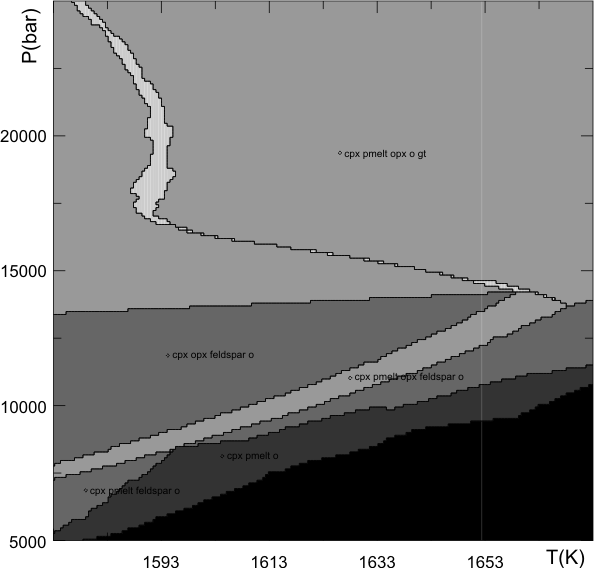
Figure 1. Melting phase relations for a simplified version of the LOSIMAG bulk mantle composition (molar composition: 0.707 SiO2, 0.037 Al2O3, 0.0971 FeO, 0.867 MgO, 0.053 CaO, 0.005 Na2O, 0.001 K2O) as a function of pressure and temperature (a). Heavy red curves depict isentropic decompression paths, labeled by entropy (J/kg), as recovered from the calculation. Olivine is stable in all phase fields. (b) Mineral and melt modes as a function of pressure along the 2565 J/kg isentrope. Absence of a spinel stability field reflects absence of Cr from the chemical model. Likewise the stability of trace amounts of sanidine (Fsp) at high pressure is an artifact of the absence of a model for K-solution in the remaining subsolidus silicates. Phase compositions where discretized with an accuracy of better than 0.03 mol% (generating 852261 pseudocompounds) on a 3-level grid with 40x40 nodes at the lowest level (157x157 nodes at the highest level).
In the following sections the prompts from Perple_X programs are written in normal font; user responses are bold font; and interspersed explanatory comments are in red. Additional explanation on some prompts is available via the (help) links.
The user/BUILD dialog that defines the calculation is reproduced with below, for more complete explanatory commentary refer to earlier tutorials:
C\jamie\Berple_X> build
NO is the default ([cr]) answer to all Y/N prompts (help)
Enter name of computational option file to be created, < 100 characters, left justified [default = in]: (help)
in20.dat
A copy of this file is at in20.dat
Enter thermodynamic data file name, left justified, [default = hp02ver.dat]: (help)
hp02ver.dat
The current data base components are:
NA2O MGO AL2O3 SIO2 K2O CAO TIO2 MNO FEO NIOO2 H2O CO2Transform them (Y/N)? (help)
n
Calculations with a saturated phase (Y/N)? (help)
The phase is: FLUID
Its compositional variable is: Y(CO2), X(O), etc.
n
Calculations with saturated components (Y/N)? (help)
n
Use chemical potentials, activities or fugacities as independent variables (Y/N)? (help)
n
Select thermodynamic components from the set: (help)
 NA2O  MGO   AL2O3 SIO2  K2O   CAO   TIO2  MNO   FEO   NIO
O2 H2O CO2 Enter names, left justified, 1 per line, <cr> to finish:SIO2
AL2O3
FEO
MGO
CAO
NA2O
K2O
The data base has P(bar) and T(K) as default independent potentials. Make one dependent on the other, e.g., as along a geothermal gradient (y/n)? (help)
n
Specify computational mode:
1 - Unconstrained minimization [default]
2 - Constrained minimization on a grid
3 - Output pseudocompound data
4 - Phase fractionation calculations
Unconstrained optimization should be used for the calculation of composition, mixed variable, and Schreinemakers diagrams, it may also be used for the calculation of phase diagram sections for a fixed bulk composition. Gridded minimization can be used to construct phase diagram sections for both fixed and variable bulk composition. Gridded minimization is preferable for the recovery of phase and bulk properties.
2
Select x-axis variable: (help)
1 - P(bar)
2 - T(K)
3 - Composition X(C1)* (user defined)
*X(C1) can not be selected as the y-axis variable
2Enter minimum and maximum values, respectively, for: T(K)
1573 1673
Select y-axis variable:
2 - P(bar)
2
This prompt is unfortunate, BUILD should "know" that the user has no choice but to put pressure on the y-axis.
Enter minimum and maximum values, respectively, for: P(bar)
5000 25000
In this mode VERTEX uses a multilevel grid to define true phase boundaries or pseudocompound assemblage boundaries, mode 1 is the most efficient, modes 2-4 should be selected if physicochemical properties are to be retrieved from the section.
Select grid refinement mode: (help)
1 - Refine only true phase boundaries, compression on.
2 - Refine only true phase boundaries, compression off [default].
3 - Refine all phase boundaries, compression on.
4 - Refine all phase boundaries, compression off.
2
Choosing mode 2 as done here represents a good general compromise between the efficiency and accuracy of the gridded minimization strategy. See the help prompt for more details.
The resolution of the grid is determined by the number of levels (JLEV) and the resolution at the lowest level in the X- and Y-directions (ILOW and JLOW, respectively), such that the maximum resolution is equivalent to that obtained on a single level grid with 1+(ILOW-1)*2^(JLEV-1) nodes in the X-direction and 1+(JLOW-1)*2^(JLEV-1) nodes in the Y-direction. To force VERTEX to use a single level grid, set JLEV=1.
Enter the number of nodes (ILOW) in the X-direction for the lowest resolution grid (0<ILOW<2048) [default = 40]: (help)
25
Enter the number of nodes (JLOW) in the Y-direction for the lowest resolution grid (1<JLOW<2048) [default = 40]: (help)
25
These choices will result in a relatively rough plot.
Enter the number of levels (JLEV) for the grid (0<JLEV<10) [default = 4]: (help)
4
These parameters define a multilevel grid equivalent to a regular X-Y grid with 195 x 195 nodes, change the parameters (y/n)?
n
Specify component amounts by weight (Y/N)?
y
Enter weight amounts of the components: (help)
SIO2 AL2O3 FEO MGO CAO K2O NA2O
for the bulk composition of interest:
45.96 4.06 7.54 37.78 3.21 0.332 0.032Do you want a print file (Y/N)?
n
Enter the plot file name, < 100 characters, left justified [default = pl]: (help)
plot20
**warning ver013** phase femg-1 has null or negative composition and will be rejected from the composition space.
Exclude phases (Y/N)? (help)
y
Do you want to be prompted for phases (Y/N)?
n
Enter phases, left justified, one per line, [cr] to finish:
lc
Do you want to treat solution phases (Y/N)?
y
Enter solution model file name [default = newest_format_solut.dat] left justified, < 100 characters: (help)
problem20_solut.dat
The above file was created by iteratively refining the compositional ranges specified for the solution models (which were also renamed) as discussed in the p-t-x pseudosection tutorial. This modified file can be copied from the link problem20_solut.dat. If you use the default solution model file, newest_format_solut.dat your results will differ from those obtained here. Do not use problem20_solut.dat for calculations outside of the P-T-X range specified here. The solution models listed below are, respectively, the pMELT melt model (Ghirso et al); clinopyroxene, orthopyroxene, olivine, garnet, spinel (all from Holland and Powell); and ternary feldspar (Fuhrman and Lindsley). Refer to the solution model glossary, or read the commentary within the solution model file itself, for more information about the solution models.
Select phases from the following list, enter 1 per line, left justified, [cr] to finish: (help)
pmelt cpx opx o gt spfeldspar
o
cpx
opx
pmelt
feldspar
gt
The solution model file defines the following dependent endmembers:
fets_i
Exclude any of these endmembers (y/n)? Answer no if you do not understand this prompt.n
Enter calculation title:
test 20
C\jamie\Berple_X> vertex
Enter computational option file name (i.e. the file created with BUILD), left justified:
in20.dat
Reading thermodynamic data from file: hp02ver.dat
Writing print output to file: none requested
Writing plot output to file: plot20
Writing pseudocompound glossary to file: pseudocompound_glossary.datReading solution models from file: problem20_solut.dat
Writing bulk composition plot output to file: bplot20
VERTEX creates an additional file named by adding a prefix "b" to the plot file name "plot20", this file, "bplot20", is needed by both PSVDRAW and WERAMI and should not be deleted or moved independently of the primary plot file. The polygon file mentioned below ("pplot20") is not used for this type of calculation.
Generating pseudocompounds, this may take a while...
... output abridged ...
Done generating pseudocompounds (total: 852261)
Because of the large number of pseudocompounds generated for the melt phase this calculation requires the "large parameter" version of VERTEX.
1.3% done with low level grid.
3.8% done with low level grid.
... output abridged ..
94.9% done with low level grid.
97.5% done with low level grid.
100.0% done with low level grid.
Beginning grid refinement stage.168 grid cells to be refined at grid level 2
refinement at level 2 involved 385 minimizations
1010 minimizations required of the theoretical limit of 2401
348 grid cells to be refined at grid level 3
...working ( 116 minimizations done)
...working ( 617 minimizations done)
refinement at level 3 involved 710 minimizations
1720 minimizations required of the theoretical limit of 9409
667 grid cells to be refined at grid level 4
...working ( 409 minimizations done)
...working ( 910 minimizations done)
refinement at level 4 involved 1265 minimizations
2985 minimizations required of the theoretical limit of 37636
If you run this example with the input files created here, you should go for a coffee break after starting VERTEX. The calculation takes about 5 hours on a 1.5 GHz PC running XP.
PSVDRAW converts the numeric data in the plot file "plot20" to PostScript graphics in the file plot20.ps; this file can be viewed in standard PostScript viewers (e.g., GhostView) or edited in most modern graphical editors (e.g., CorelDraw or Illustrator).
C\jamie\Berple_X> psvdraw
Enter the Perple_X plot file name: plot20PostScript will be written to file: plot20.ps
Modify the default plot (y/n)?
n
The postscript output is plotted below (Figure 2).
Figure 2. Computed phase relations as output by PSVDRAW.
The compositional limits and resolution for the pmelt model in problem20_solut.dat were refined prior to the calculation illustrated here. Iterative refinement of solution models is an important aspect of using Perple_X and is discussed in the p-t-x pseudosection tutorial.
To extract the adiabat (isentrope) the user first runs WERAMI to create a P-T-entropy surface:
C\jamie\Berple_X> weramiEnter the VERTEX plot file name:plot20Select operational mode:1 - compute properties at specified conditions2 - create a property grid (plot with pscontor)3 - compute properties along a curve or line (plot with pspts)4 - as in 3, but input from file2Select a property:1 - Specific Enthalpy (J/m3)2 - Density (kg/m3)... output abridged...17 - Entropy (J/K/kg)18 - Enthalpy (J/kg)19 - Heat Capacity (J/K/kg)20 - Specific mass of a phase (kg/m3-solid)17Calculate individual phase properties (y/n)? nChange default variable range (y/n)? nEnter number of nodes in and x and y directions: (help)50 50Writing grid data to file: cplot20Range of >0 data is: 2487.57 -> 2702.21Evaluate additional properties (y/n)? n
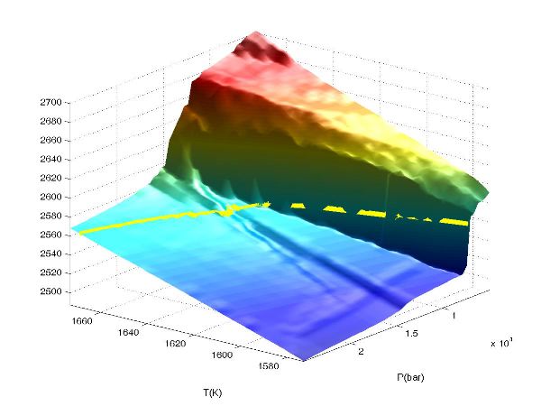
The preceding dialog generates a new plot/data file cplot20 that defines entropy as a function of pressure and temperature. This data can be plotted using the Perple_X program PSCONTOR or MatLab as illustrated in the seismic velocity tutorial. The dialog below demonstrates the use of PSCONTOR to recover a the pressure-temperature coordinates of a single contour (specifically the 2565 J/kg isentrope, Figure 1) [this entire procedure is much simpler in MatLab]:
C\jamie\Berple_X> pscontorEnter the CONTOUR plot file name:cplot20PostScript will be written to file: cplot20.psReset plot limits (y/n)? nModify default drafting options (y/n)?answer yes to modify:- picture transformation- x-y plotting limits- relative lengths of axes- text label font size- line thickness- curve smoothing- axes labeling and gridding nContoured variable range 2487.569 -> 2702.211Modify default contour interval (y/n)?yEnter min, max and interval for contours:2565 2565 1Echo contour data to file contor.dat (Y/N)?y
Figure 3. Entropy (J/kg) as a function of pressure and temperature as obtained by WERAMI and plotted in MatLab. The yellow curve shows the 2565 J/kg isentrope as defined in revised_contor.dat, because of interpolation error the contour makes small excursions from the entropy surface.
The file "contor.dat" defines the contour in a series of segments that generally are not sequential and are separated by text. To process this data so that it can be used as input for subsequent calculations import it into a spread-sheet program (such as Excel) and sort it first to eliminate the text, and second to order the coordinates along the contour. Note that the coordinates must be sorted by pressure, because temperature does not decrease continuously along the 2565 J/kg isentrope (Figure 1) and that temperature (X) and pressure (Y) must be in the first column of the revised file. The file created by such processing has been named "revised_contor.dat". In principle revised_contor.dat could now be used as an input file in WERAMI to recover properties along the contour; however the highly irregular entropy surface (Figure 3) creates some difficulties that can be circumvented by refining the contour data. The difficulties arise because small interpolation errors associated with defining the contour can lead to a large error in the real value of the entropy if the entropy surface has large gradients (i.e., if you are on the face of a cliff a small variation in your horizontal position can have disastrous implications for your elevation). Such irregularities may be real, as for example the rapid increase in entropy associated with melting in the plagioclase lherzolite field; but smaller irregularities may also result because WERAMI does not interpolate (although it does extrapolate) between grid points. As a consequence there are steps between the representative areas associated with the grid nodes (these are not visible in Figure 3, but can be seen if a higher resolution grid, e.g., 400x400, is used to recover the entropy surface). To filter out contour coordinates that do not lie on the surface being contoured, it is wise to run WERAMI a second time to check the real value of the property along the contour does not differ from the nominal value the contour is intended to represent. The WERAMI dialog for this procedure is:
C\jamie\Berple_X> weramiEnter the VERTEX plot file name:plot20Select operational mode:1 - compute properties at specified conditions2 - create a property grid (plot with pscontor)3 - compute properties along a curve or line (plot with pspts)4 - as in 3, but input from file4Select a property:1 - Specific Enthalpy (J/m3)2 - Density (kg/m3)... output abridged...17 - Entropy (J/K/kg)18 - Enthalpy (J/kg)19 - Heat Capacity (J/K/kg)20 - Specific mass of a phase (kg/m3-solid)17Calculate individual phase properties (y/n)? nChange default variable range (y/n)? nCalculate individual phase properties (y/n)?Writing profile to file: cplot20Path will be described by:1 - a file containing a polynomial function2 - a file containing a list of x-y pointsEnter 1 or 2 (default=2):2Enter the file name:revised_contor.datFile contains 1301 points, every nth plot will be plotted, enter n:11573.00 7318.19 2566.651573.04 7319.18 2566.681573.39 7334.50 2572.691573.50 7336.94 2572.78...output abridged...1668.98 24892.9 2565.001668.99 24898.0 2565.001668.99 24899.4 2565.001668.99 24899.4 2565.001668.99 24901.9 2565.001669.09 24976.8 2565.001669.13 24999.9 2565.00 Evaluate additional properties (y/n)?n
The each row of the file cplot20 created by WERAMI now consists of a symbol code (that can be deleted), the X (temperature) coordinate, the entropy value, and the Y (pressure) coordinate. This file can in turn be imported into a spread-sheet program (e.g., Excel) and the rows sorted according to the entropy coordinate. Rows associated with entropy values that differ significantly from the nominal entropy of the contour (2565 J/kg) are then deleted, and the columns reordered so that temperature and pressure are, respectively, in the first and second columns, and the data sorted by the pressure coordinate. The file generated by such processing in this example is "final_contor.dat", and can be used to recover properties such as modal proportions along the contour as in the dialog below:
C\jamie\Berple_X> weramiEnter the VERTEX plot file name:plot20Select operational mode:1 - compute properties at specified conditions2 - create a property grid (plot with pscontor)3 - compute properties along a curve or line (plot with pspts)4 - as in 3, but input from file4Select a property:1 - Specific Enthalpy (J/m3)2 - Density (kg/m3)3 - Specific heat capacity (J/K/m3)4 - Expansivity (1/K, for volume)5 - Compressibility (1/bar, for volume)6 - Weight percent of a component7 - Mode (Vol %) of a compound or solution8 - Composition of a solution9 - Grueneisen thermal ratio10 - Adiabatic bulk modulus11 - Shear modulus (bar)12 - Sound velocity (km/s)13 - P-wave velocity (Vp, km/s)14 - S-wave velocity (Vs, km/s)15 - Vp/Vs16 - Specific Entropy (J/K/m3)17 - Entropy (J/K/kg)18 - Enthalpy (J/kg)19 - Heat Capacity (J/K/kg)20 - Specific mass of a phase (kg/m3-solid)7Enter solution or compound name (left justified):pmeltWriting profile to file: cplot20Path will be described by:1 - a file containing a polynomial function2 - a file containing a list of x-y pointsEnter 1 or 2 (default=2):2Enter the file name: final_contor.datFile contains 686 pointsevery nth plot will be plotted, enter n:11573.00 7318.19 23.62811573.04 7319.18 23.62801595.89 8517.59 15.46431595.67 8528.55 15.46371597.62 8625.20 15.0290... output abridged ... because the Perple_X plotting routines will not label the curves its worth noting the range of the mode (the third value here) to help you identify which curves correspond to which mineral.
1668.99 24901.9 0.2901001669.09 24976.8 0.2900311669.13 24999.9 0.290010Evaluate additional properties (y/n)?y... by answering yes here, the mode of the additional phases (i.e., o, opx, cpx, feldspar, gt) may be collected in the same file (cplot20).
The plot file cplot20 generated by the preceeding dialog can be plotted directly with the Perple_X program PSPTS. Alternatively (my preference), the data can be converted with the Perple_X program PT2CURV to a format that can be plotted with PSVDRAW:
C\jamie\Berple_X> pt2curvin file?cplot20out file?pr20_modesC\jamie\Berple_X> psvdrawEnter the Perple_X plot file name:pr20_modesPostScript will be written to file:pr20_modes.psModify the default plot (y/n)?yModify default drafting options (y/n)?answer yes to modify:- picture transformation- x-y plotting limits- relative lengths of axes- text label font size- line thickness- curve smoothing- axes labeling and griddingyModify x-y limits (y/n)? nModify default picture transformation (y/n)?nModify ratio of x to y axis length (y/n)nModify default text scaling (y/n)?nUse minimum width lines (y/n)?nFit curves with B-splines (y/n)?yRestrict phase fields by variance (y/n)?answer yes to:- suppress pseudounivariant curves and/or pseudoinvariant points nRestrict phase fields by phase identities (y/n)?answer yes to:- show fields that contain a specific assemblage- show fields that do not contain specified phases- show fields that contain any of a set of specified phasesnModify default equilibrium labeling (y/n)?answer yes to:- modify/suppress [pseudo-] univariant curve labels- suppress [pseudo-] invariant point labelsnEnd-of-file! if this is a VERTEX plot file then VERTEX terminated incorrectlyModify default axes (y/n)?yEnter the starting value and interval for major tick marks onthe X-axis (the current values are: 0.732E+04 0.354E+04)Enter the new values:10000 5000Enter the starting value and interval for major tick marks onthe Y-axis (the current values are: 0.00 13.3 )Enter the new values:0 10Cancel half interval tick marks (y/n)? nDraw tenth interval tick marks (y/n)? nRescale axes text (y/n)? nTurn gridding on (y/n)?n
The resulting plot is shown below (Figure 4).
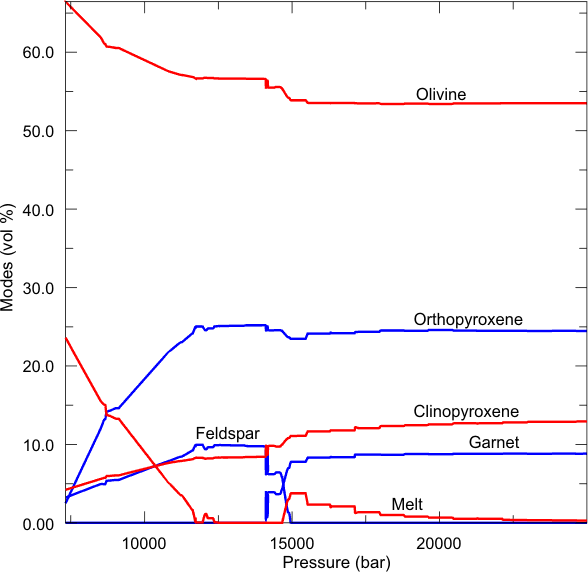
Figure 4. Modes along the 2565 J/kg adiabat as output by PSVDRAW (curve and axes relabeled and color added).