NOTE: MU_2_F is obsolete in
Perple_X
'07 because activities and fugacities can be specified as computational
variables.
This document is an updated "on-line" version example 6 of the Perple_X documentation; this is hardly a brilliant example, but I don't have time to make a new one. My reason for updating this example is to illustrate a new Perple_X program MU_2_F for converting phase diagram calculated as a function of chemical potentials to diagrams as a function of activities or fugacities. For those users hoping for the long promised chapter 10 of the tutorial, my apologies, this web page is not it.
ai = exp [{Gi(P,T)-Goi(P,T)}/R/T]where Goi(P,T) is the molar Gibbs energy of the pure species i at the temperature and pressure of interest, Gi(P,T) is the molar Gibbs energy of the species i at the temperature, pressure and concentration of interest, and R is the universal gas constant. In contrast, fugacities are defined as:
fi(P,T) = fi(Pr,T) exp [{Gi(P,T)-Goi(Pr,T)}/R/T]where Goi(Pr,T)is the molar Gibbs energy of the pure species i at the reference pressure and temperature of interest, where the factor fi(Pr,T) is included to account for the possibility that the standard state (e.g., an ideal gas) at the reference pressure and temperature is not the stable state (e.g., a real gas).
The relation between fugacity or activity and the chemical potential
of the component i ("ui") follows from the above relations
from the constraint that at equilibrium Gi(P,T)
= ui.
This example differs from the previous ones in that chemical potentials are used as independent variables, a difficulty in such calculations is that often users have no idea what range of chemical potential values are appropriate for a calculation. In this case there are two possible approaches, either one calculates an initial phase diagram for a very wide range of chemical potentials, and then examines and refines interesting regions of the resulting diagram; or one calculates limits on the chemical potentials based on saturation values and activity models. FRENDLY is useful for defining the range of chemical potential of interest, this application is illustrated below. Note that VERTEX will not recognize saturation of a mobile component (in fact this would be inconsistent with its algorithm), and so it is the users responsibility to ascertain that reasonable limits are used.
For the present problem, which is perhaps relevant to skarn formation, pressure and temperature are assumed (T = 863 K, P = 2000 bar). The first task is to estimate the range of u(SiO2) of interest. The upper limit is defined by quartz saturation, and the lower limit as the Gibbs energy of quartz with some reduced activity, say 0.01 (alternatively a "low" u(SiO2) could be obtained by taking the Gibbs energy for the reaction En - Fo at 863 K and 2000 bar). The oxygen chemical potential "u(O2)" must also be specified, and is taken to be that corresponding to log f(O2) = -10 (oxidizing conditions). Alternatively, COHSRK or FRENDLY could be used to calculate a limit on u(O2) from fluid speciation or phase equilibria (e.g., QFM), or better still to create a buffer for u(O2) consistent with some fluid composition or heterogenous equilibria, such as QFM, as a function of P and T (see Documentation Section 1.4, Example 1.4).
Note that many of the fluid equations of state included in Perple_X
do not take account of the effects of u(O2) on fluid speciation; in which
case, as here, the results will may only be valid under (oxidizing) conditions
at which the fluid can be assumed to be essentially a binary H2O-CO2 mixture.
Here the user runs FRENDLY to get u(SiO2) and u(O2) (i.e., the
molar Gibbs energy quartz and ideal oxygen gas). In FRENDLY the default
answer to yes/no questions is no.
c\thermo>frendlythe program starts by asking some irritating questions for various historical reasons.Enter the thermo data file name, left justified, < 15 characters
(default = hp98ver.dat):
hp98ver.datHi! i am a user freindly program. What is your name?
j
Hi j !, i like you and i hope we have fun!
Can you say "therm-o-dy-nam-ics" (y/n)?
y
Choose from following options:1 - calculate equilibrium coordinates for a reaction.
2 - calculate thermodynamic properties for a phase or reaction relative to the reference state.
3 - calculate change in thermodynamic properties from one p-t-x condition to another.
4 - create new thermodynamic data file entries.
5 - quit.
With options 1-3 you may also modify thermodynamic data, modified data can then be stored as a new entry in the thermodynamic data file."q" is the abbreviation for quartz in Holland and Powell's (1998) data base, refer to the header of the data file for a complete list of abbreviations and other information on the data base.
2
List database phases (y/n)?
n
Calculate thermodynamic properties for a reaction (y/n)?
n
Calculate thermodynamic properties for phase:
qThe value of G here is the saturation value for q, i.e., disregarding kinetic problems, the upper limit on the chemical potential of silica at 863 K and 2000 bar.
Enter activity of: q (enter 1.0 for H2O or CO2):
1
standard state properties follow:g(j/mole) s(j/mole k) v(j/mole bar)
-856464.60 41.500000 2.2688000heat capacity (j/mole k) function:
a b*t c/t^2 d*t^2 e/t^(1/2)
110.70000 -0.51890000E-02 0.0000000 0.0000000 -1128.3000f/t g/t**3
0.0000000 0.0000000parameters b1-b8 for the volumetric (j/mole bar) function (see program documentation Eqs 2.1-2.3):
0.65000000E-05 0.0000000 0.0000000 0.0000000 -0.65000000E-04
783541.90 -112.50000 4.0000000The phase or reaction has a transition-dependent function.
Super function for g (j/mole):
-837901.19 829.06530 2.2694959 110.70000 -0.25945000E-02
0.0000000 0.0000000 -4513.2000 0.0000000 0.0000000
0.14747200E-04 0.0000000 0.0000000 0.0000000 -0.29494400E-03
783541.90 -112.50000 4.0000000j write a properties table (Y/N)?
n
Now j , there is one thing i want you to remember and that is that the values for G and H are "apparent" free energies and enthalpies. j if you dont know what that means read Helgeson et al. 1978. j now i am going to prompt you for conditions at which i should calculate thermodynamic properties, when you want to stop just enter zeroes. ok, here we go, it is fun time j !!Enter p(bars) and t(k) (zeroes to quit):
2000 863
At 863.000 k and 2000.00 bar:
G(kj) = -895.00237To get a lower limit on u(SiO2), the user must now lower the activity of quartz and recalculate its molar Gibbs energy.
H(kj) = -804.05907
A(kj) = -899.68307
U(kj) = -808.73977
S(j/k) = 105.380
V(j/bar)= 2.34035
Cp(j/k) = 80.4404
loge K = 124.733
log10 K = 54.1709Modify or output thermodynamic parameters (y/n)?
y
Do you only want to output data (y/n)?
n
Thermodynamic properties are calculated from the reference state constants G, S, V, and an activity coefficient together with the isobaric heat capacity function:
The name chosen here has no significance.cp(pr,t) = a + b*t + c/t^2 + d*t^2 + e/t^(1/2) + f/t + g/t^3and the volumetric function:if b8 = 0 (Eq 2.1):
v(p,t) = v(pr,tr) + b2(t-tr) + b4(p-pr) + b6(p-pr)^2 + b7(t-tr)^2if b8 < 0 (Eq 2.2):v(p,t) = v(pr,tr) exp [b3*(t-tr) + b8*(p-pr)]if b8 > 0 (Eq 2.3):v(p,t) = v(pr,t)[1 + b8*p/(Kt + b8*p)]^(1/b8)Enter the number of the parameter to be modified:
alpha = b1 + b2*t + b3/t + b4/t^2 + b5/t^(1/2)
Kt = b6 + b7*t1) standard free energy g (j) 2) standard entropy s (j/k)
3) standard volume v (j/bar) 4) heat capacity coefficient a
5) heat capacity coefficient b 6) heat capacity coefficient c
7) heat capacity coefficient d 8) heat capacity coefficient e
9) heat capacity coefficient f 10) heat capacity coefficient g
11) volumetric coefficient b1 12) volumetric coefficient b2
13) volumetric coefficient b3 14) volumetric coefficient b4
15) volumetric coefficient b5 16) volumetric coefficient b6
17) volumetric coefficient b7 18) volumetric coefficient b8
19) activity 20) reaction coefficiententer zero when you are finished:
19
Enter a name (<8 characters left justified) to distinguish the modified version of q . WARNING: if you intend to store modified data in the data file this name must be unique.
q1This prompt is only relevant for reactions, that it is given at this point is due to a bug.
Old value for activity of q1 was 1.0000000
Enter new value:
0.01
Enter the number of the parameter to be modified:1) standard free energy g (j) 2) standard entropy s (j/k)
3) standard volume v (j/bar) 4) heat capacity coefficient a
5) heat capacity coefficient b 6) heat capacity coefficient c
7) heat capacity coefficient d 8) heat capacity coefficient e
9) heat capacity coefficient f 10) heat capacity coefficient g
11) volumetric coefficient b1 12) volumetric coefficient b2
13) volumetric coefficient b3 14) volumetric coefficient b4
15) volumetric coefficient b5 16) volumetric coefficient b6
17) volumetric coefficient b7 18) volumetric coefficient b8
19) activity 20) reaction coefficiententer zero when you are finished:
0
Store q1 as an entry in data file hp98ver.dat (y/n)?
n
Modify properties of another phase (y/n)?
nThe value of G here is taken as the lower value of silica chemical potential for the phase diagram calculation, i.e., the phase diagram will be computed for a range of chemical potentials corresponding to quartz activity between 1 (saturation) and 0.01.
Enter p(bars) and t(k) (zeroes to quit):
2000 863
At 863.000 k and 2000.00 bar:
G(kj) = -928.04603The user must now exit to the main menu, to repeat the procedure just executed for silica for oxygen.
H(kj) = -804.05907
A(kj) = -932.72672
U(kj) = -808.73977
S(j/k) = 143.670
V(j/bar)= 2.34035
Cp(j/k) = 80.4404
loge K = 129.338
log10 K = 56.1709
Modify or output thermodynamic parameters (y/n)?
nChoose from following options:
Enter p(bars) and t(k) (zeroes to quit):
0 0
1 - calculate equilibrium coordinates for a reaction.To save time the user can specify an activity or fugacity different from unity at the outset of the calculation, note that in most geological thermodynamic data bases gaseous species properties are not assigned a pressure dependence, this means that the property reported by FRENDLY for such species as Goi(P,T) is in fact Goi(Pr,T), and thus the property entered here is the fugacity. In some cases, most notably for H2O and CO2, Perple_X has routines that permit calculation of both Goi(P,T) and Goi(Pr,T), in which case the user is free to choose between activity and fugacity.
2 - calculate thermodynamic properties for a phase or reaction relative to the reference state.
3 - calculate change in thermodynamic properties from one p-t-x condition to another.
4 - create new thermodynamic data file entries.
5 - quit.
With options 1-3 you may also modify thermodynamic data, modified data can then be stored as a new entry in the thermodynamic data file.
2
List database phases (y/n)?
n
Calculate thermodynamic properties for a reaction (y/n)?
n
Calculate thermodynamic properties for phase:
O2
Enter activity of: O2 (enter 1.0 for H2O or CO2):
1e-10
standard state properties follow:g(j/mole) s(j/mole k) v(j/mole bar)
0.0000000 205.20000 0.0000000
heat capacity (j/mole k) function:The value of G is the chemical potential of O2 for the phase diagram calculation, i.e., corresponding to a log10(fO2) = -10.a b*t c/t^2 d*t^2 e/t^(1/2)
48.300000 -0.69100000E-03 499200.00 0.0000000 -420.70000f/t g/t**3
0.0000000 0.0000000parameters b1-b8 for the volumetric (j/mole bar) function (see program
documentation Eqs 2.1-2.3):0.0000000 0.0000000 0.0000000 0.0000000 0.0000000
0.0000000 0.0000000 0.0000000super function for g (j/mole):
63013.244 164.00877 0.0000000 48.300000 -0.34550000E-03
249600.00 0.0000000 -1682.8000 0.0000000 0.0000000
0.0000000 0.0000000 0.0000000 0.0000000 0.0000000
0.0000000 0.0000000 0.0000000j write a properties table (Y/N)?
n
Now j , there is one thing i want you to remember and that is that the values for G and H are "apparent" free energies and enthalpies. j if you dont know what that means read Helgeson et al. 1978. j now i am going to prompt you for conditions at which i should calculate thermodynamic properties, when you want to stop just enter zeroes. ok, here we go, it is fun time j !!Enter p(bars) and t(k) (zeroes to quit):
2000 863
At 863.000 k and 2000.00 bar:
G(kj) = -291.92643
H(kj) = 79.142858
A(kj) = -291.92643
U(kj) = 79.142858
S(j/k) = 429.976
V(j/bar)= 0.00000
Cp(j/k) = 34.0520
loge K = 40.6847
log10 K = 17.6691Modify or output thermodynamic parameters (y/n)?
n
Enter p(bars) and t(k) (zeroes to quit):
0 0
Choose from following options:1 - calculate equilibrium coordinates for a reaction.
2 - calculate thermodynamic properties for a phase or reaction relative to the reference state.
3 - calculate change in thermodynamic properties from one p-t-x condition to another.
4 - create new thermodynamic data file entries.
5 - quit.With options 1-3 you may also modify thermodynamic data, modified data can then be stored as a new entry in the thermodynamic data file.
5
Have a nice day j !
The user is now armed with a range of values for u(SiO2) (-928046
to -895002 j/mol-SiO2) and a value for u(O2) (-291926 j/mol-O2). The next
step is to run BUILD to prepare the input for VERTEX.
This dialog should be relatively transparent for users who have worked through the tutorial or example files, and is therefore reproduced here with minimal commentary.
c\jamie\perplex_f90>build
NO is the default ([cr]) answer to all Y/N prompts
Enter name of computational option file to be created, < 100 characters, left justified [default = in]:
in6.dat
Enter thermodynamic data file name, left justified, [default = hp98ver.dat]:
hp98ver.dat
The current data base components are:
NA2O MGO AL2O3 SIO2 K2O CAO TIO2 MNO FEO O2 H2O CO2
Transform them (Y/N)?
n
Calculations with a saturated phase (Y/N)?
The phase is: FLUID
Its compositional variable is: Y(CO2), X(O), etc.
y
Select the independent saturated phase components:
H2O CO2
Enter names, left justified, 1 per line, [cr] to finish:
For C-O-H fluids it is only necessary to select volatile species present in the solids of interest. If the species listed here are H2O and CO2, then to constrain O2 chemical potential to be consistent with C-O-H fluid speciation treat O2 as a saturated component. Refer to the Perple_X Tutorial for details.
H2O
CO2
Calculations with saturated components (Y/N)?
n
Use chemical potentials, activities or fugacities as independent variables (Y/N)?
y
Chemical potentials are symbolized in Perple_X, by a lowercase u followed by the component name in parentheses, e.g., the potential of A is written u(A).
To convert chemical potentials to activities or fugacities run the Perple_X program MU_2_F after running VERTEX (see on-line documentation for additional information).
Select < 3 mobile components from the set:
NA2O MGO AL2O3 SIO2 K2O CAO TIO2 MNO FEO O2
Enter names, left justified, 1 per line, [cr] to finish:
O2
SIO2
Select thermodynamic components from the set:
NA2O MGO AL2O3 K2O CAO TIO2 MNO FEO
Enter names, left justified, 1 per line, [cr] to finish:
AL2O3
CAO
FEO
Select fluid equation of state:
0 - X(CO2) Modified Redlich-Kwong (MRK/DeSantis/Holloway)
1 - X(CO2) Kerrick & Jacobs 1981 (HSMRK)
2 - X(CO2) Hybrid MRK/HSMRK
3 - X(CO2) Saxena & Fei 1987 pseudo-virial expansion
4 - Bottinga & Richet 1981 (CO2 RK)
5 - X(CO2) Holland & Powell 1991, 1998 (CORK)
6 - X(CO2) Hybrid Haar et al 1979/CORK (TRKMRK)
7 - f(O2/CO2)-f(S2) Graphite buffered COHS MRK fluid
8 - f(O2/CO2)-f(S2) Graphite buffered COHS hybrid-EoS fluid
9 - Max X(H2O) GCOH fluid Cesare & Connolly 1993
10 - X(O) GCOH-fluid hybrid-EoS Connolly & Cesare 1993
11 - X(O) GCOH-fluid MRK Connolly & Cesare 1993
12 - X(O)-f(S2) GCOHS-fluid hybrid-EoS Connolly & Cesare 1993
13 - X(H2) H2-H2O hybrid-EoS
14 - EoS Birch & Feeblebop (1993)
15 - X(H2) low T H2-H2O hybrid-EoS
16 - X(O) H-O HSMRK/MRK hybrid-EoS
17 - X(O) H-O-S HSMRK/MRK hybrid-EoS
18 - X(CO2) Delany/HSMRK/MRK hybrid-EoS, for P > 10 kb
19 - X(O)-X(S) COHS hybrid-EoS Connolly & Cesare 1993
20 - X(O)-X(C) COHS hybrid-EoS Connolly & Cesare 1993
21 - X(CO2) Halbach & Chatterjee 1982, P > 10 kb, hybrid-Eos
22 - X(CO2) DHCORK, hybrid-Eos
23 - Toop-Samis Silicate Melt
5
The data base has P(bars) and T(K) as default independent potentials.
Make one dependent on the other, e.g., as along a geothermal gradient (y/n)?
n
Specify computational mode:
1 - Unconstrained minimization [default]
2 - Constrained minimization on a grid
3 - Output pseudocompound data
Unconstrained optimization should be used for the calculation of composition,
mixed variable, and Schreinemakers diagrams, it may also be used for the
calculation of phase diagram sections for a fixed bulk composition. Gridded
minimization can be used to construct phase diagram sections for both fixed
and variable bulk composition. Gridded minimization is preferable for the
recovery of phase and bulk properties.
1
Specify number of independent potential variables:
0 - Composition diagram [default]
1 - Mixed-variable diagram
2 - Sections and Schreinemakers-type diagrams
2
Select x-axis variable:
1 - P(bars)
2 - T(K)
3 - Y(CO2)
4 - u(O2)
5 - u(SIO2)
3
Enter minimum and maximum values, respectively, for: Y(CO2)
0 0.8
Select y-axis variable:
2 - T(K)
3 - P(bars)
4 - u(O2)
5 - u(SIO2)
5
Enter minimum and maximum values, respectively, for: u(SIO2)
Be careful with negative numbers, BUILD may not stop you from entering a minimum value > your maximum value, but this will cause VERTEX to write an error message and stop.
...output abridged...-928046 -895002
Specify sectioning value for: P(bars)
2000
Specify sectioning value for: u(O2)
-291926
Specify sectioning value for: T(K)
863
Constrain bulk composition (as in pseudosections, y/n)?
n
Do you want a print file (Y/N)?
y
Enter the print file name, < 100 characters, left justified [default = pr]:
print6
Long print file format (Y/N)?
n
Write full reaction equations (Y/N)?
n
Suppress console status messages (Y/N)?
n
Print dependent potentials for chemographies (Y/N)?
Answer no if you do not know what this means.
n
Do you want a plot file (Y/N)?
y
Enter the plot file name, < 100 characters, left justified [default = pl]:
plot6
Specify efficiency level [1-5, default = 3]:
1 - gives lowest efficiency, highest reliability
5 - gives highest efficiency, lowest reliability
High values increase probability that a curve may be partially determined or skipped.
3
**warning ver013** phase iron has null or negative composition and will be
rejected from the composition space.
**warning ver013** phase gph has null or negative composition and will be
rejected from the composition space.
**warning ver013** phase diam has null or negative composition and will be
rejected from the composition space.
**warning ver013** phase CO has null or negative composition and will be
rejected from the composition space.
**warning ver013** phase CH4 has null or negative composition and will be
rejected from the composition space.
**warning ver013** phase H2 has null or negative composition and will be
rejected from the composition space.
Exclude phases (Y/N)?
n
Do you want to treat solution phases (Y/N)?
y
Enter solution model file name [default = solut.dat]
left justified, < 100 characters:
solut.dat
**warning ver113** F is not a valid model because component H2O or CO2 is cons
**warning ver025** 1 endmembers for MnCtd The solution will not be considered.
Select phases from the following list, enter 1 per line,
left justified, [cr] to finish
F Chl T hCrd TrTs TrTsPg
GlTrTs GCOHF H2OM CzEpPs EpCz Opx(HP)
Cpx(l) Cpx(h) GrAd(EW) GrAd GrPyAlSp(B GrPyAlSp(G
GrPyAl(G) GtD Gt(HP) GrPyAl(B) trgltsch Mn-Opx(HP)
MnChl
The calculation illustrated here is simplified by consideration of only two mineral solutions, grandite and epidote. For a more rigorous calculation, the user might consider a more complex epidote model (i.e., CzEpPs) as well as models for clinpyroxene, amphibole. The "art" of using Perple_X is in the choice of solution models, to do this properly there is no alternative to actually reading the comments in the solution model file to discover the purpose of a particular model.
Because of the above simplification both univariant and pseudounivariant equilibria can be displayed without resulting in a completely illegible diagram (interpretaion of pseudo-univariant equilibria is discussed various papers [Connolly and Kerrick 1987 CALPHAD, Connolly 1990 AJS, Connolly and Trommsdorff 1991 CMP], in the Perple_X Tutorial Chaps 4 and 9, and partially in the pseudosection tutorial). Consequently the user requests that pseudounivariant equilibria are calculated, the calculation could be simplified further by answering no here (alternatively the pseudounivariant curves can be suppressed in PSVDRAW as shown later in this example).GrAd
EpCz
Calculate high variance phase fields (Y/N)?
y
Enter a title for your calculation:
Test Problem 6
The user dialog with VERTEX is self-explanatory:VERTEX
c\jamie\thermo>vertex
Enter computational option file name (i.e. the file created with BUILD), left justified:
in6.dat
Reading thermodynamic data from file: hp98ver.dat
Writing print output to file: print6
Writing plot output to file: plot6
cycle 1 1 1
...output abridged...
cycle 11 20 21
Initial number of divariant assemblages to be tested is: 21
Testing divariant assemblage 1, 20 assemblages remaining to be tested.
finished with equilibrium ( 1) cor cc = GrAd(gr)
finished with equilibrium ( 2) cor GrAd(gr) = an
finished with equilibrium ( 3) cor cc = an
finished with equilibrium ( 4) cc an = GrAd(gr)
finished with equilibrium ( 5) cor cc GrAd(gr80) = GrAd(gr89)
...output abridged...
Testing divariant assemblage 68, 1 assemblages remaining to be tested.
Testing divariant assemblage 69, 1 assemblages remaining to be tested.
Testing divariant assemblage 70, 0 assemblages remaining to be tested.
c\thermo>mu_2_fMU_2_F does not overwrite the original plot file, but instead it creates a new plot file that is named by adding the prefix "m" to the original plot file name.
Enter the VERTEX plot file name:
plot6
the new plot file will be named: mplot6
MU_2_F analyzes the plot file to determine which, if any, of the variables can be converted.
convert u(SIO2) to activity (or fugacity) (y/n)?Whether the chemical potential is converted to an activity or fugacity is dependent upon the identity of the species chosen for the conversion.
y
the converted variable will be named: lf_SIO2 and is the base 10 log of the activity (or fugacity).
Enter the thermo data file name, left justified, < 15 charactersThe same data base should be used for the conversion as was used for the original calculation.
(default = hp98ver.dat):
hp98ver.datHere the user most specify the thermodynamic species used to define the activity or fugacity of silica from its chemical potential. In general, this must be a species with the same composition as the component to which the chemical potential corresponds, and by convention it is usually the species that would be stable (or at least dominant) in a system composed entirely of the component at the pressure and temperature of interest, i.e., in the present case quartz:
List database phases (y/n)?
n
Select a phase or species to be used to define lf_SIO2 (default =SIO2 )
qFor solid phase species, as here, MU_2_F converts the chemical potential to an activity. In the case of a fluid species for which Perple_X has a built-in equation of state, MU_2_F would offers the user the option of converting to either activity or fugacity, otherwise MU_2_F converts to fugacities.
c\thermo>psvdrawNote that this is not the VERTEX plot file, rather the file generated by MU_2_F
Enter the VERTEX plot file name:
mplot6
PostScript will be written to file: mplot6.ps
Modify the default plot (y/n)?
y
Modify default drafting options (y/n)?
answer yes to modify:
- picture transformation
- x-y plotting limits
- relative lengths of axes
- text label font size
- line thickness
- curve smoothing
- axes labeling and gridding
y
Modify x-y limits (y/n)?
n
Modify default picture transformation (y/n)?
n
Modify ratio of x to y axis length (y/n)
n
Modify default text scaling (y/n)?
n
Use minimum width lines (y/n)?
n
Fit curves with B-splines (y/n)?
y
Restrict phase fields by variance (y/n)?
answer yes to:
- suppress pseudounivariant curves or pseudoinvariant points
n
Restrict phase fields by phase identities (y/n)?
answer yes to:
- show fields that contain a specific assemblage
- show fields that do not contain specified phases
- show fields that contain any of a set of specified phases
n
Modify default equilibrium labeling (y/n)?
answer yes to:
- modify/suppress [pseudo-] univariant curve labels
- suppress [pseudo-] invariant point labels
n
Modify default axes (y/n)?
y
Enter the starting value and interval for major tick marks on
the X-axis (the current values are: 0.00 0.160 )
Enter the new values:
0 0.2
Enter the starting value and interval for major tick marks on
the Y-axis (the current values are: -2.00 0.400 )
Enter the new values:
-2 0.5
Cancel half interval tick marks (y/n)?
n
Draw tenth interval tick marks (y/n)?
n
Rescale axes text (y/n)?
n
Turn gridding on (y/n)?
n
c\thermo>psvdrawNote that this is not the VERTEX plot file, rather the file generated by MU_2_F
Enter the Perple_X plot file name:
mplot6This means curves longer than 10% of the axes length receive a text label:
PostScript will be written to file: mplot6.ps
Modify the default plot (y/n)?
y
Modify default drafting options (y/n)?
answer yes to modify:
- picture transformation
- x-y plotting limits
- relative lengths of axes
- text label font size
- line thickness
- curve smoothing
- axes labeling and gridding
y
Modify x-y limits (y/n)?
n
Modify default picture transformation (y/n)?
n
Modify ratio of x to y axis length (y/n)
n
Modify default text scaling (y/n)?
n
Use minimum width lines (y/n)?
n
Fit curves with B-splines (y/n)?
y
Restrict phase fields by variance (y/n)?
answer yes to:
- suppress pseudounivariant curves or pseudoinvariant points
y
Suppress pseudounivariant curves (y/n)?
y
Suppress pseudoinvariant points (y/n)?
n
Restrict phase fields by phase identities (y/n)?
answer yes to:
- show fields that contain a specific assemblage
- show fields that do not contain specified phases
- show fields that contain any of a set of specified phases
n
Modify default equilibrium labeling (y/n)?
answer yes to:
- modify/suppress [pseudo-] univariant curve labels
- suppress [pseudo-] invariant point labels
y
Suppress curve labels (y/n)?
n
Change default labeling of curve segments (y/n)?
y
Suppress labels of pseudounivariant curves (y/n)?
y
Enter minimum fraction of the axes length that a
curve must be to receive a text label (0-1):
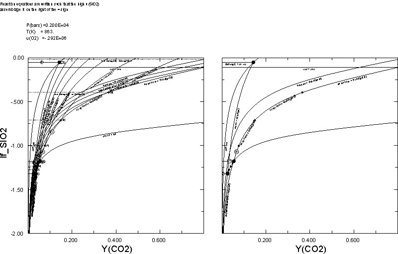
0.1and curves longer than 2%, and less than 10%, of the axes length receive a numeric label, shorter curve segments are not labeled.
Enter minimum fraction of the axes length that a
curve must be to receive a numeric label (0-0.100):
0.02The plots on the right and left are those generated by Dialog 1 and 2, respectively. An interesting point demonstrated here is that increasing a chemical potential has a similar effect to increasing the thermal potential, hence the qualitative similarity of the calculated u(SiO2)-YCO2 diagram with the more common T-YCO2 diagram.
Suppress point labels (y/n)?
y
Modify default axes (y/n)?
y
Enter the starting value and interval for major tick marks on
the X-axis (the current values are: 0.00 0.160 )
Enter the new values:
0 0.2
Enter the starting value and interval for major tick marks on
the Y-axis (the current values are: -2.00 0.400 )
Enter the new values:
-2 0.5
Cancel half interval tick marks (y/n)?
n
Draw tenth interval tick marks (y/n)?
n
Rescale axes text (y/n)?
n
Turn gridding on (y/n)?
n
PSVDRAW Output