!!!WARNING!!!
This tutorial is for an out-of-date version of Perple_X (Perple_X 06), the best current tutorial for the calculation of phase diagram sections is the seismic velocity tutorial. Although the seismic velocity tutorial illustrates the extraction of seismic velocities from a phase diagram section, the basic procedure is typical of phase diagram section calculations. The tutorial here has not been removed because components of this tutorial illustrate features, e.g., 1-d phase fractionation and the specification of pressure-temperature paths for phase diagram calculations, that are still pertinent to the current version of Perple_X and not addressed in other Perple_X tutorials.
IntroductionRunning BuildRunning VertexRunning PsvdrawRunning Werami in Mode 1Plotting Mineral Modes with WERAMI, PT2CURV and PSVDRAWFigures:Figure 1. Metapelite phase diagram section with fractionation pathFigure 2. Phase relations during fractionationFigure 3. Mineral modes with and without fractionation
This is a bare bones tutorial intended to illustrate phase fractionation calculations in Perple_X. In phase fractionation calculations the initial bulk composition of a system, and a path that defines the evolution of the systems physical conditions, are specified. The program VERTEX computes the initial stable assemblage for the specified bulk composition and increments the systems conditions along the path. After each increment the program "removes" all phases that are to be fractionated by adjusting the systems composition and recalculates the stable phase assemblage. The formation of refractory garnet porphyroblasts or the loss of a mobile fluid, or melt, phase are typical scenarios where fractionation calculations are relevant. In the limit that the incremental steps along the systems path become infinitely small, fractionation calculations are identical to Rayliegh fractionation.
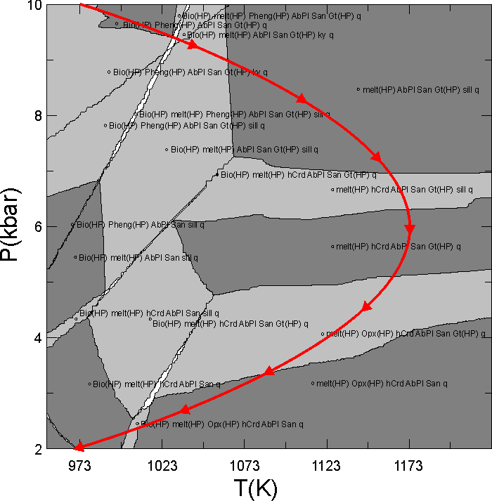
This document illustrates a calculation in which the granitic melt that forms during heating and decompression of a pelitic rock is fractionated from the bulk composition. The phase diagram section (pseudosection) for the initial bulk composition is shown in Figure 1. The problem of concern here is to compute phase relations along the P-T path depicted by the red curve in Figure 1 if melt generated during decompression from 10 to 6 kbar is instantaneously removed from the system. The calculation done here is made with the haplogranitic melt model described by White et al. (2001, JMG); however melt fractionation calculations can also be done in Perple_X using the MELTs and PMELTS model of Ghiorso and Sack (1995, CMP) and Ghirso et al. (2002, G3).
Figure 1. Calculated phase relations for Shaw's (1956) average metapelitic bulk composition. This section was calculated using gridded minimization as detailed in the phase diagram section calculation of the seismic velocity tutorial; the input file for the phase diagram calculation is ain18.dat, and that for the fractionation calculation is in18.dat.
The type of calculation required for this example is a minor variation on the pseudosection calculations described in detail in the pseudosection and the seismic velocity tutorials. Novice users should refer to these tutorials for more complete explanation of the various prompts and methods used here.
In the following sections the prompts from Perple_X programs are written in normal font; user responses are bold font; and interspersed explanatory comments are in red.
The user/BUILD dialog that defines the fractionation calculation is reproduced with commentary below:
c\jamie\Berple_X> build
NO is the default ([cr]) answer to all Y/N prompts
In this context, "default" is what Perple_X assumes if the user simply presses the enter key in response to a prompt.
Enter name of computational option file to be created,
< 100 characters, left justified [default = in]:
Enter thermodynamic data file name, left justified, [default = hp02ver.dat]:
hp02ver.dat
The current data base components are:
NA2O MGO AL2O3 SIO2 K2O CAO TIO2 MNO FEO NIO ZRO2 CL2O2 H2O CO2Transform them (Y/N)?
n
Calculations with a saturated phase (Y/N)?
The phase is: FLUID
Its compositional variable is: Y(CO2), X(O), etc.
n
H2O cannot be specified as a saturated phase or saturated component for calculations with any of the silicate melt models currently available in Perple_X (i.e., melt(HP), MELTs(GS), and PMELTS(G)). Despite this, users can force water saturation by specifying a large amount of H2O component in the bulk composition.
Calculations with saturated components (Y/N)?
n
Use chemical potentials, activities or fugacities as independent variables (Y/N)?
n
Select thermodynamic components from the set:
NA2O MGO AL2O3 SIO2 K2O CAO TIO2 MNO FEO NIO ZRO2 CL2O2 H2O CO2Enter names, left justified, 1 per line, [cr] to finish:
NA2O
MGO
AL2O3
SIO2
K2O
CAO
FEO
H2O
Regardless of whether melt is present or not, for phase fractionation calculations in which fluid is fractionated the fluid components must be specified as thermodynamic components.
**warning ver016** you are going to treat a saturated (fluid) phase component as a thermodynamic component, this may not be what you want to do.
Select fluid equation of state:
0 - X(CO2) Modified Redlich-Kwong (MRK/DeSantis/Holloway)1 - X(CO2) Kerrick & Jacobs 1981 (HSMRK)2 - X(CO2) Hybrid MRK/HSMRK3 - X(CO2) Saxena & Fei 1987 pseudo-virial expansion4 - Bottinga & Richet 1981 (CO2 RK)5 - X(CO2) Holland & Powell 1991, 1998 (CORK)6 - X(CO2) Hybrid Haar et al 1979/CORK (TRKMRK)7 - f(O2/CO2)-f(S2) Graphite buffered COHS MRK fluid8 - f(O2/CO2)-f(S2) Graphite buffered COHS hybrid-EoS fluid9 - Max X(H2O) GCOH fluid Cesare & Connolly 199310 - X(O) GCOH-fluid hybrid-EoS Connolly & Cesare 199311 - X(O) GCOH-fluid MRK Connolly & Cesare 199312 - X(O)-f(S2) GCOHS-fluid hybrid-EoS Connolly & Cesare 199313 - X(H2) H2-H2O hybrid-EoS14 - EoS Birch & Feeblebop (1993)15 - X(H2) low T H2-H2O hybrid-EoS16 - X(O) H-O HSMRK/MRK hybrid-EoS17 - X(O) H-O-S HSMRK/MRK hybrid-EoS18 - X(CO2) Delany/HSMRK/MRK hybrid-EoS, for P > 10 kb19 - X(O)-X(S) COHS hybrid-EoS Connolly & Cesare 199320 - X(O)-X(C) COHS hybrid-EoS Connolly & Cesare 199321 - X(CO2) Halbach & Chatterjee 1982, P > 10 kb, hybrid-Eos22 - X(CO2) DHCORK, hybrid-Eos23 - Toop-Samis Silicate Melt
5
The data base has P(bar) and T(K) as default independent potentials. Make one dependent on the other, e.g., as along a geothermal gradient (y/n)?
n
The present calculation requires such a dependence, however for phase fractionation calculations the user gets a second chance to define a dependence; therefore it is not necessary to answer yes here.
Specify computational mode:
1 - Unconstrained minimization [default]
2 - Constrained minimization on a grid
3 - Output pseudocompound data
4 - Phase fractionation calculations
Unconstrained optimization should be used for the calculation of composition, mixed variable, and Schreinemakers diagrams, it may also be used for the calculation of phase diagram sections for a fixed bulk composition. Gridded minimization can be used to construct phase diagram sections for both fixed and variable bulk composition. Gridded minimization is preferable for the recovery of phase and bulk properties.
4
Fractionation calculations are path dependent, select path type:
1 - path with variable P(bar), all other variables constant2 - path with variable T(K), all other variables constant3 - path with P(bar) = f(T(K)), all other variables constant4 - path with T(K) = f(P(bar), all other variables constant5 - arbitrary user specified coordinates4
Here it is desired to fractionate along the curved red path in Figure 1, thus options 3 or 4 are in principal possible. In Perple_X the independent variable must be increase or decrease continuously; thus the choice of pressure as the independent variable allows calculations along the entire path shown in Figure 1, whereas a P = f(T) would require that the user do the user do the calculation of the entire path in two pieces, i.e., one in which T is increasing (P > 6 kbar) and a second in which T is decreasing (P < 6 kbar). After having done this calculation I realized that melting stops along the cooling portion of P-T path, so the calculations done here are only at P > 6 kbar and in this case option 3 is as good as 4. In fact, the Perple_X plotting program, PSVDRAW, behaves (draws tick marks, etc) better if the independent variable increases along the fractionation path, so actually option 3 would be preferable here.
In mode 5 VERTEX prompts the user for each physical condition interactively. The Perple_X graphics programs cannot be used in conjunction with mode 5 calculations.
The dependence must be described by the polynomial
T(K) = Sum ( c(i) * [P(bar)]^i, i = 0..n)
In Perple_X paths are defined by a polynomial of the form
Y = c0 + c1 X1 + c2 X2 + ... + cn Xn
where Y is the dependent path variable, X is the independent path variable, c0 ... cn are the polynomial coefficients and n is the order of the polynomial. The next prompts define the fractionation path as a function of the independent variable (P); to this end the path in Figure 1 was fit to a second order polynomial to obtain:
T(K) = 723 + 0.15 P(bar) - 1.25e-5 P(bar)2
Such fitting is easily done in programs such as Excel, Mathematica, or Maple.
Enter n (<5)
2
Enter c( 0)
623
Enter c( 1)
0.15
Enter c( 2)
-1.25e-5
Enter start and end values, respectively, for: P(bar)
10000 6000
How many points along the path?
400
In the limit that the number of points along the P-T path is large fractionation calculations in Perple_X approximate Rayleigh ("equilibrium") fractionation. There is no simple rule for what a "large" number of points is, so users should increase the number of points until the results cease depending on the number of points requested (at which point the calculation simulates Rayleigh fractionation). Because of the pseudocompound approximation, Perple_X results have an inherent roughness that cannot be eliminated by increasing the number of points used; however this roughness can be reduced by increasing the number of pseudocompounds used to represent solution phases.
Specify component amounts by weight (Y/N)?
n
Enter molar amounts of the components:
NA2O MGO AL2O3 SIO2 K2O CAO FEO H2O
for the bulk composition of interest:
3.16 5.73 17 105.7 3.56 2.21 9.05 7.
Here the user specifies the initial composition of the system in terms of molar amounts of the components. These quantities define a "mole" of the system, i.e., one mole of the system contains 7 moles of H2O, 3.16 moles of NA2O, etc.
The amount of water was chosen here so that the system was not fluid saturated at the initial condition (Figure 1). The initial water content has a profound influence on the phase relations.
Do you want a print file (Y/N)?
y
In contrast to most complex Perple_X calculations, the print file for fractionation calculations is not so large as to be incomprehensible and may be useful for some users. Provided the user requests assemblage data (as in the 2nd prompt below), the print file contains a list of all the assemblages and their physical properties along the specified fractionation path. The assemblages are output after each increment along the fractionation path before the phase or phases to be fractionated have been removed.
Enter the print file name, < 100 characters, left justified [default = pr]:
print18
Print pseudodivariant assemblage data (y/n)?
y
Print dependent potentials for chemographies (Y/N)?
Answer no if you do not know what this means.
Do you want a plot file (Y/N)?
y
Enter the plot file name, < 100 characters, left justified [default = pl]:
plot18
**warning ver013** phase femg-1 has null or negative composition and will be rejected from the composition space.
Exclude phases (Y/N)?
n
Do you want to treat solution phases (Y/N)?
y
Enter solution model file name [default = newest_format_solut.dat] left justified, < 100 characters:
newest_format_solut.dat
**warning ver025** 0 endmembers for MELTS(GS) The solution will not be considered.
...output abridged...
**warning ver025** 1 endmembers for Ep(HP) The solution will not be considered.
Select phases from the following list, enter 1 per line,
left justified, [cr] to finish
MnBio(HP) Bio(HP) Chl(HP) MnChl(HP) O(SG) E(SG)
Omph(HP) Cpx(HP) melt(HP) pMELTS(G) Opx(HP) Pheng(HP)
Sapp(HP) GaHcSp T MnSt(HP) Ctd(HP) Carp
hCrd Sud(Livi) Sud Cumm Anth Gl
Tr TrTsPg(HP) GlTrTs GlTrTsPg feldspar Pl(h)
AnPl AbPl Ab(h) Ab Kf(h) Kf
San MaPa KN-Phen MuCel PaCel MuPa
Pa Mu O(HP) Cpx(l) Cpx(h) Mont
Sp(JR) Sp(GS) Sp(HP) Neph(FB) GrPyAlSp(B GrPyAlSp(G
Gt(HP) GrPyAl(B) A-phase Chum Atg B
P Qpx Mn-Opx OrFsp(C1) AbFsp(C1) Pl(I1,HP)
Fsp(C1) MuPaMa(CH)
AbPl
San
Pheng(HP)
Bio(HP)
hCrd
Gt(HP)
TrTsPg(HP)
melt(HP)
Sapp(HP)
MnSt(HP)
Opx(HP)
AnPl
O(HP)
Sp(HP)
Pa
The solution model file defines the following dependent endembers:
mnts_i sdph_i fame_i fafchl_i mame_i mafchl_i fets_i
fsp4_i ftat_i hfcrd_i hmncrd_i fparg_i fts_i fgl_i
ncel_i nfcel_i
Exclude any of these endmembers (y/n)?
Answer no if you do not understand this prompt.n
Enter calculation title:
Fractionation test
In contrast to other computational modes, in fractionation calculations VERTEX requires more interaction than simply specification of the input file.
c\jamie\Berple_X> vertex
Enter computational option file name (i.e. the file created
with BUILD), left justified:in18.dat
Reading thermodynamic data from file: hp02ver.dat
Writing print output to file: print18Writing plot output to file: plot18
Writing pseudocompound glossary to file: pseudocompound_glossary.dat
Reading solution models from file: newest_format_solut.dat
Writing bulk composition plot output to file: bplot18Initializing polygon output file: pplot18
VERTEX creates an additional file named by adding a prefix "b" to the plot file name "plot18", this file, "bplot18", is needed by both PSVDRAW and WERAMI and should not be deleted or moved independently of the primary plot file. The polygon file mentioned below ("pplot18") is not used for this type of calculation.
Generating pseudocompounds, this may take a while...
Endmember configurational entropies (doc. eq. 8.2) for Bio(HP) are:
phl - 11.52622 ann - 11.52622 east - 0.00000
sdph_i - 0.00000
1678 pseudocompounds generated for: Bio(HP)
**warning ver041** icky pseudocompound names for solution model: melt(HP)
refer to pseudocompound_glossary.dat file for pseudocompound definitions.
649460 pseudocompounds generated for: melt(HP)
Because of the large number of pseudocompounds generated for the melt phase this calculation requires the "large parameter" version of VERTEX.
... output abridged ...
**warning ver114** the following endmembers are missing for Gt(HP)
spss
Endmember configurational entropies (doc. eq. 8.2) for Gt(HP) are:
alm - 0.00000 py - 0.00000 gr - 0.00000
1222 pseudocompounds generated for: Gt(HP)
Done generating pseudocompounds (total: 670029)
Fractionate phases (y/n)?y
If the user answers no to this prompt, VERTEX calculates the stable (non-fractionated) phase relations along the fractionation path.
Enter the name of a phase to be fractionated (left justified, [cr] to finish):
melt(HP)
VERTEX writes a file named by appending the suffix ".dat" to each phase to be fractionated that contains a record of the molar amount and composition of fractionated phases. Thus in the present case, a record of the melt amount and composition is in melt(HP).dat. In this file the first number is the value of the independent path variable at which fractionation occurred, the second number is the number of moles of the phase, the third entry is the phase name, and the remaining numbers are the amounts of the systems components removed by the fractionation (i.e., the composition of the fractionated phase). These amounts are listed in the same order as the components are output in mode 1 calculations with WERAMI (see below).
Here the user specifies the phases to be fractionated, these may be either solutions (solid, fluid, or melt) or stoichiometric phases (e.g., quartz, water). More than one phase may be fractionated. BEWARE: fractionation may completely eliminate one or more components from the bulk composition, when this occurs VERTEX may give erratic results, in which case the fractionation should be restarted at the point at which the component disappears with the depleted component eliminated from the bulk composition specified in the input file. The unstable behavior occurs because VERTEX always defines the system in terms of as many stable pseudocompounds as there are specified components, even if the amount of the component is zero. Thus if water becomes depleted (as is the case here) VERTEX will still identify a pseudocompound that contains water as a stable phase, but will set the amount of this phase to zero. As the amount of the phase is zero, any water-bearing phase can be chosen without affecting the total energy of the system or violating the mass balance constraints for the system. In general VERTEX does choose a phase that would be stable if the amount of the component were vanishingly small (rather than zero).
Enter the name of a phase to be fractionated
(left justified, [cr] to finish):
At P(bar) = 10000.0 and T(K) = 973.000
melt(HP) is not stable.
... output abridged ...
VERTEX writes progress diagnostics to the users console; here these indicate that between 10000 and 9398.50 bar the melt is not stable.
At P(bar) = 9398.50 and T(K) = 1028.63
melt(HP) is not stable.
At P(bar) = 9385.96 and T(K) = 1029.69
fractionating 1.38442 moles of melt(HP); changes bulk by:
0.692211 0.00000 0.232583 2.30368 0.116291 0.00000 0.00000 0.116291
Once the phase to be fractionated becomes stable VERTEX reports the amount of the phase that formed since the last increment and the change in the systems composition that results from removal of the phase (the amounts of the components are listed in the same order as the components are output in mode 1 calculations with WERAMI (see below).
At P(bar) = 9373.43 and T(K) = 1030.75
fractionating 5.39750 moles of melt(HP); changes bulk by:
2.69875 0.00000 0.982346 8.83031 0.453390 0.151130 0.00000 0.377825
At P(bar) = 9360.90 and T(K) = 1031.80
fractionating 3.50699 moles of melt(HP); changes bulk by:
1.75349 0.00000 0.638272 5.73743 0.294587 0.981957E-01 0.00000 0.245489
At P(bar) = 9348.37 and T(K) = 1032.86
fractionating -.569345E-15 moles of melt(HP); changes bulk by:
-.284673E-15 0.00000 -.103621E-15 -.931449E-15 -.478250E-16 -.159417E-16 0.00000 -.398542E-16
... output abridged ...
At P(bar) = 8947.37 and T(K) = 1064.41
fractionating 0.00000 moles of melt(HP); changes bulk by:
0.00000 0.00000 0.00000 0.00000 0.00000 0.00000 0.00000 0.00000
At 8947 bar melt fractionation has completely depleted water from the bulk composition and at this point the caveat mentioned above becomes operative. Thus VERTEX identifies the melt as the stable phase that would form if a vanishingly small amount of water were present, but because water is depleted, the amount of melt is zero. Accordingly its "fractionation" does not affect the bulk composition. Another way of thinking of this situation is that at the conditions where the melt is identified as stable, but absent, the stable phases are saturated (but not oversaturated) with respect to a melt phase.
... output abridged ...
At P(bar) = 6979.95 and T(K) = 1161.00
fractionating 0.00000 moles of melt(HP); changes bulk by:
0.00000 0.00000 0.00000 0.00000 0.00000 0.00000 0.00000 0.00000
At 6967 bar melt is no longer stable, subsequent analysis of the output (with WERAMI) shows that cordierite (hCrd) becomes the saturated water-bearing phase at lower pressures.
At P(bar) = 6967.42 and T(K) = 1161.30
melt(HP) is not stable.
... output abridged ...
At P(bar) = 6015.04 and T(K) = 1173.00
melt(HP) is not stable.
At P(bar) = 6002.51 and T(K) = 1173.00
melt(HP) is not stable.
Perple_X treats fractionation calculations as a special case of gridded minimization in which the Y-grid variable corresponds to the independent variable of the fractionation path and the X-grid variable is assigned a value of zero; thus the output of fractionation calculations can be plotted in PSVDRAW and analyzed with WERAMI as a 2-dimensional grid that is one node wide. The basic plot obtained by running PSVDRAW is crude (Figure 2), but useful for identifying the stable phases along the fractionation path (again with the caveat that one or more phases may be present with zero amount).
c\jamie\Berple_X> psvdraw
Enter the Perple_X plot file name:plot18
PostScript will be written to file: plot18.ps
PSVDRAW converts the numeric data in plot18 to PostScript graphics in the file plot18.ps; this file can be viewed in standard PostScript viewers (e.g., GhostView) or edited in most modern graphical editors (e.g., CorelDraw or Illustrator).
Modify the default plot (y/n)?
n
** warning ** you are plotting a 1-dimensional grid as a 2-dimensional plot. The width of the X-axis is arbitrary, the assigned value for the X-axis variable is: 0.00000

Figure 2. Simplified phase relations along the fractionation path, the amount of melt in the melt + AbPl + San + Gt + sill + q field is zero, likewise the amount of cordierite (hCrd) in the hCrd + AbPl + San + Gt + sill + q field is zero. To make the plot legible the phase relations have been simplified at pressures corresponding to the onset of melting where the coincidence of the fractionation path with a corner of the Bio + Pheng + AbPl + San + Gt + q field (Figure 1) creates complexities that are not easily resolved on the scale of the diagram. Because the Y-axis increases downward PSVDRAW does not place tick marks on the vertical axis. Note that the "temperature" axis is retained only for plotting, but has no significance (the temperature is determined by the pressure along the fractionation curve).
As is the case for any gridded minimization in Perple_X the plot file output by VERTEX for fractionation calculations can be analyzed directly with (plot18) WERAMI. In this regard it is relevant to observe that WERAMI records the abundances of phases computed after conditions have been incremented along the fractionation path, but before the phases have been fractionated; thus the amount of a phase that is undergoing fractionation may be greater than zero. The user/WERAMI dialog to extract mineral modes and the fractionated bulk composition at 9200 bar along the fractionation path is reproduced below:
C\jamie\Berple_X>werami
Enter the VERTEX plot file name:plot18
** warning ** you are plotting a 1-dimensional grid as a 2-dimensional plot. The width of the X-axis is arbitrary, the assigned value for the X-axis variable is: 0.00000
Select operational mode:
1 - compute properties at specified conditions
2 - create a property grid (plot with pscontor)
3 - compute properties along a curve or line (plot with pspts)
4 - as in 3, but input from file1
Console output will be echoed in file: rplot18
The "echo" file is sometimes useful because it can be used to print or read the wide tables generated by WERAMI in a more legible format. On most operating systems users can also adjust the width of the console to make the console output from WERAMI more comprehensible.
Enter T(K) and P(bar) (zeroes to quit):
0.001 9200
The only trick to remember in running WERAMI for fractionation calculations is that WERAMI, like PSVDRAW, "thinks" the X variable corresponds to temperatures (or whatever the dependent path variable is) in the range 0-0.001.
 ---------
 (   80) Stable phases at:
                             T(K)     = 0.100000E-02
                             P(bar)   =  9200.00
                                                       Molar Phase Compositions:
                    mol%  wt%   vol%(2) H2O   MGO   AL2O3 SIO2  K2O   CAO   FEO   NA2O
 Bio(HP)(Bi65_62)   2.17  6.95  6.80    1.00  1.71  0.88  2.62  0.50  0.00  0.92  0.00
 melt(HP)(me622681) 0.39  0.39  0.50    0.50  0.00  0.18  1.64  0.08  0.03  0.00  0.07
 AbPl(an29)         4.78  9.12 10.01    0.00  0.00  0.65  2.70  0.00  0.30  0.00  0.35
 AbPl(an31)         3.44  6.57  7.21    0.00  0.00  0.65  2.69  0.00  0.31  0.00  0.34
 San(sa75)          8.89 17.44 19.81    0.00  0.00  0.50  3.00  0.38  0.00  0.00  0.12
 Gt(HP)(a65p29)     6.82 22.79 16.42    0.00  0.89  1.00  3.00  0.00  0.13  1.98  0.00
 sill               7.06  8.18  7.31    0.00  0.00  1.00  1.00  0.00  0.00  0.00  0.00
 q                 66.46 28.56 31.93    0.00  0.00  0.00  1.00  0.00  0.00  0.00  0.00
The mineral modes reported here can be used to check if a phase that is reported to be stable is actually present. E.g., for this problem the mode of melt(HP) is found to be zero at pressures below that of the biotite stability field drawn with PSVDRAW (Figure 2), likewise the mode of cordierite is zero within the "hCrd" stability field.
                         Molar Properties(2):
                      N(g)      H(J)    V(J/bar) Cp(J/K) Alpha(1/K)   Beta(1/bar) Density(kg/m3)
 Bio(HP)(Bi65_62)   446.86 -0.49648E+07  15.113  551.42  0.35812E-04  0.20304E-05   2956.9
 melt(HP)(me622681) 139.69 -0.16999E+07  6.2225  216.65  0.84010E-04  0.45199E-05   2244.9
 AbPl(an29)         266.96 -0.34265E+07  10.126  315.96  0.24265E-04  0.15981E-05   2636.4
 AbPl(an31)         267.20 -0.34308E+07  10.125  316.07  0.24073E-04  0.15893E-05   2639.0
 San(sa75)          274.39 -0.33562E+07  10.767  313.91  0.21688E-04  0.18037E-05   2548.4
 Gt(HP)(a65p29)     467.55 -0.47558E+07  11.639  509.42  0.26942E-04  0.64538E-06   4017.2
 sill               162.03 -0.22343E+07  5.0077  198.56  0.14833E-04  0.83423E-06   3235.6
 q                   60.09 -0.77458E+06  2.3216  86.262  0.15632E-03  0.50444E-05   2588.3
 System            8180.20 -0.98935E+08  282.64  10107.  0.65398E-02  0.22279E-03

                         Seismic (Molar) Properties(2):
                      Gruneisen     Ks(bar)     Mu(bar)    V0(km/s)     Vp(km/s)    Vs(km/s)
 Bio(HP)(Bi65_62)     0.48340     0.49251E+06   0.0000      4.0812      0.0000      0.0000
 melt(HP)(me622681)   0.53383     0.22124E+06   0.0000      3.1393      0.0000      0.0000
 AbPl(an29)           0.48659     0.62574E+06   0.0000      4.8718      0.0000      0.0000
 AbPl(an31)           0.48523     0.62921E+06   0.0000      4.8830      0.0000      0.0000
 San(sa75)            0.41244     0.55441E+06   0.0000      4.6643      0.0000      0.0000
 Gt(HP)(a65p29)       0.95379     0.15495E+07   0.0000      6.2106      0.0000      0.0000
 sill                 0.44843     0.11987E+07   0.0000      6.0866      0.0000      0.0000
 q                    0.83403     0.19824E+06   0.0000      2.7675      0.0000      0.0000
Shear moduli and seismic properties that depend on the shear modulus are only reported if the thermodynamic data file includes data for the endmember shear moduli, this is not generally the case. See the seismic velocity tutorial for more information.
Bulk Composition:

                mol     mol %      wt %
    H2O        1.39     1.11      0.31
    MGO        5.73     4.57      2.82
    AL2O3     15.00    11.97     18.70
    SIO2      87.25    69.61     64.10
    K2O        2.62     2.09      3.01
    CAO        1.98     1.58      1.36
    FEO        9.05     7.22      7.94
    NA2O       2.33     1.86      1.77
The absolute molar composition output by WERAMI (2nd column above) is particularly useful in fractionation calculations because the difference between this composition and the initial composition specified for the problem gives the integrated composition of the fractionated phase; e.g., at this point in the calculation the system contains 1.39 mole H2O, as the system initially contained 7 mole H2O, fractionation has removed 5.61 mole H2O.
Bulk Properties:Density (kg/m3) (2) = 2894.2 Specific Enthlpy (J/m3) (2) = -.350035E+11 Specific Heat Capacity (J/K/m3) (1) = 0.357583E+07 Aggregate Grueneisen Ratio (2,3) = 0.621984 Aggregate Adiabatic Bulk Modulus (bar) (2,3) = 523433. Aggregate Shear Modulus (bar) (2,3,4) = 0.00000 Aggregate Sound Velocity (km/s) (2,3) = 4.25273 Aggregate P-Wave Velocity (km/s) (2,3,4) = 0.00000 Aggregate S-Wave Velocity (km/s) (2,3,4) = 0.00000 Variance (c-p+2) = 0 Notes: 1 - Computed at reference condition (P(bar) = 9218., T(K) =1044.). 2 - Computed from linearized equation of state relative to the reference condition. 3 - Computed by Voigt-Reuss-Hill scheme (e.g., Bina & Helfrich 1992). 4 - If zero, shear modulus data is not in the data base. --------- Enter T(K) and P(bar) (zeroes to quit):
Bulk and phase properties of the stable assemblage can be plotted with computational modes 2, 3, and 4 in WERAMI, for 1-dimensional calculations such as mode 3 is preferable because users can extract several properties in a single run. The dialog reproduced below illustrates the extraction of mineral modes along the fractionation path with WERAMI.
C\jamie\Berple_X> werami
Enter the VERTEX plot file name:plot18
** warning ** you are plotting a 1-dimensional grid as a 2-dimensional plot. The width of the X-axis is arbitrary, the assigned value for the X-axis variable is: 0.00000
Select operational mode:
1 - compute properties at specified conditions
2 - create a property grid (plot with pscontor)
3 - compute properties along a curve or line (plot with pspts)
4 - as in 3, but input from file3
Select a property:
1 - Specific enthalpy (J/m3)
2 - Density (kg/m3)
3 - Specific Heat capacity (J/K/m3)
4 - Expansivity (1/K, for volume)
5 - Compressibility (1/bar, for volume)
6 - Weight percent of a component
7 - Mode (Vol %) of a compound or solution
8 - Composition of a solution
9 - Grueneisen thermal ratio
10 - Adiabatic bulk modulus
11 - Shear modulus (bar)
12 - Sound velocity (km/s)
13 - P-wave velocity (Vp, km/s)
14 - S-wave velocity (Vs, km/s)
15 - Vp/Vs7
Enter solution or compound name (left justified):
San
Include fluid in computation of aggregate (or modal) properties (y/n)?
n
Writing profile to file:
cplot18
WERAMI generates a new plot file, named by adding the prefix "c" to the VERTEX plot file name "plot18", this new file is the file that is used by any subsequent plotting (e.g., PSPTS) or conversion (e.g., PT2CURV) programs.
Enter endpoint 1 (T(K) -P(bar) ) coordinates:
0.0001 10000
Again, recollect that the "T(K)" variable has no meaning and has been assigned a range from 0 to 0.001 by WERAMI (or perhaps VERTEX?).
Enter endpoint 2 (T(K) -P(bar) ) coordinates:
0.0001 6000
How many points along the profile?
200
There is no reason to specify a number greater than the number of increments used in the fractionation calculation (400 here); but ideally the number of points should be close to the number of increments so that the profile accurately portrays the data (a lower value is used in this example only to save space).
P(bar) T(K) Property
10000.0 0.100000E-03 1.39114
9979.90 0.100000E-03 1.41827
9959.80 0.100000E-03 1.41820
9939.70 0.100000E-03 1.41812
Because the Perple_X plotting programs do not identify the properties that are plotted it is useful to useful to note the range of the properties reported by WERAMI as an aid to interpreting the ultimate plotted output. Alternatively, once a plot has been constructed, WERAMI can be used in Mode 1 for this purpose.
6080.40 0.100000E-03 27.3014
6060.30 0.100000E-03 27.3016
6040.20 0.100000E-03 27.3019
6020.10 0.100000E-03 27.3021
Evaluate additional properties (y/n)?y
By answering yes, the user can choose the mode of additional phases, so that all the modal data is collected in the file cplot18.
The plot file cplot13 generated by WERAMI can be plotted directly with PSPTS, which plots a symbol at each data point. I personally do not like this type of plot, but the PSPTS dialog is reproduced below:
C\jamie\Berple_X> pspts
Enter the POINT plot file name:
cplot18
PostScript will be written to file: cplot18.ps
Modify the default plot (y/n)?
n
The plot file cplot13 generated by WERAMI can be converted to a format that can be plotted with PSVDRAW by running the program PT2CURV as follows:
C\jamie\Berple_X> pt2curv
in file?
cplot18
out file?
mplot18
The name of the output file (to be plotted with PSVDRAW) can be whatever the user finds convenient.
The converted plot file can be plotted without modification in PSVDRAW, the dialog below a few modifications of the default plot are specified to improve the cosmetics of the basic PostScript plot:
C\jamie\Berple_X> psvdraw
Enter the Perple_X plot file name:
mplot18
PostScript will be written to file: mplot18.psModify the default plot (y/n)?
y
Modify default drafting options (y/n)?
answer yes to modify:
- picture transformation
- x-y plotting limits
- relative lengths of axes
- text label font size
- line thickness
- curve smoothing
- axes labeling and griddingy
Modify x-y limits (y/n)?
y
Enter new min and max for X old values were: 6000.0 10000.
6000 10000
Enter new min and max for Y old values were: -1.0000 35.015
0 36
OK, but this may look sloppy.
Modify default picture transformation (y/n)?
n
Modify ratio of x to y axis length (y/n)
n
Modify default text scaling (y/n)?
n
Use minimum width lines (y/n)?
n
Fit curves with B-splines (y/n)?
y
Restrict phase fields by variance (y/n)?
answer yes to:
- suppress pseudounivariant curves and/or pseudoinvariant pointsn
Restrict phase fields by phase identities (y/n)?
answer yes to:
- show fields that contain a specific assemblage
- show fields that do not contain specified phases
- show fields that contain any of a set of specified phasesn
Modify default equilibrium labeling (y/n)?
answer yes to:
- modify/suppress [pseudo-] univariant curve labels
- suppress [pseudo-] invariant point labelsn
End-of-file! if this is a VERTEX plot file then VERTEX terminated incorrectly
Modify default axes (y/n)?
y
Enter the starting value and interval for major tick marks on the X-axis (the current values are: 0.600E+04 800. )
Enter the new values:6000 1000
Enter the starting value and interval for major tick marks on the Y-axis (the current values are: 0.00 7.20 )
Enter the new values:0 10
Cancel half interval tick marks (y/n)?
n
Draw tenth interval tick marks (y/n)?
n
Rescale axes text (y/n)?
n
Turn gridding on (y/n)?
n
This plot was then modified (to change line styles and add colors) in a graphics program (CorelDraw) and superimposed on the results of a calculation of the phase relations along the fractionation path without fractionation to obtain Figure 3.
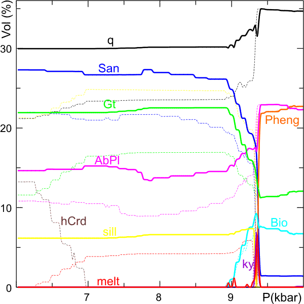
Figure 3. Phase volume proportions with (heavy solid curves) and without (thin dashed curves) melt fractionation during decompression from 10 to 6 kbar along the P-T path indicated in Figure 1. The final result of this calculation shows that the fractionation of a small amount of melt has a surprisingly large effect on the modal proportions and the final stable assemblage. This is primarily due to the water depletion caused by melt fractionation. It is interesting that, both with and without fractionation, melting initiates during the breakdown of hydrated silicates (Biotite and Phengite) and that once these water sources are exhausted there is no significant (none?) melt production with decompression and heating. In fact, to the contrary, in the calculation without fractionation, melt crystallizes during heating after Cordierite begins to compete with the melt for water.