Perple_X Equilibrium Reactive-Transport
Calculations: TITRATE Model Configuration
Contents
Steps in a
TITRATE calculation
Thoughts on
configuring/running a TITRATE calculation
Explanation/Definition of Variables
Figures:
Figure 1: FRAC2D vs TITRATE
reactive transport model geometry
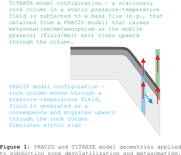
Perple_X is configured to do two general types of equilibrium
reactive transport models, FRAC2D
and TITRATE (Figure 1). Both
configurations are referred to within Perple_X
as 2d-phase fractionation models (Connolly 2005).
In these calculations a 1-dimensional column of rock is subject to
perturbations that lead to the formation of one or more mobile phases (e.g.,
melt and low-density electrolytic or molecular fluids). The rate at which the
perturbations are applied adds a second effective dimension, time, to the
model. The mobile phase(s), i.e., fractionated phase, moves upward through the
column until it is consumed or passes through the top of the column. The two
types of calculations are distinguished by the mechanism for perturbing the
initial equilibrium condition: in FRAC2D calculations, the perturbation is
caused by changing pressure-temperature conditions, as occurs within a
subducted slab or during regional metamorphism; in TITRATE calculations the
perturbation is a mass flux across the base of the column, as occurs in the
mantle wedge during subduction and other metasomatic processes. This page
documents the TITRATE configuration,
refer to the FRAC2D page for an outline of
the FRAC2D configuration. FRAC2D and TITRATE represent limiting cases, the
intermediate case in which the column moves through a dynamic P-T field and is
simultaneously subject to a basal mass flux can be computed as a variant of the
FRAC2D configuration in which the TITRATE variable (see below for definition of all input/output
variables) is set.
The
input files for the TITRATE example outlined here are at www.perplex.ethz.ch/perplex/examples/TITRATE
are designated by the project name titrate.
The fractionated, or mobile phase, is represented by the solution model
COH-Fluid+, a model for low-density C-O-H-S fluids. Depending on the aq_lagged_speciation option specified in the Perple_X option file, COH-Fluid+ may represent
either molecular or electrolytic fluids (Connolly and
Galvez, 2018). The example here uses the molecular version of the model and
thus corresponds to an up-date of the subduction model used by Connolly (2005). It is
advisable to work with the molecular model before attempting the electrolytic
model which introduces additional complexity and uncertainty. As in all Perple_X calculations, the project name has no
special significance, the name titrate used here is chosen solely for purpose of the
example. In this example, equilibrium phase relations are computed for a 50 m
tall column of ultramafic rock, the base of which is at the mantle-wedge/slab
interface at a depth of 128 km, and within which temperature rises upward. The
depth corresponds to that at which the slab interface in the FRAC2D example (frac2d_noaq.dat)
is subject to a large fluid flux as a consequence of slab devolatilization. The
chemical composition of the fluxes used in the TITRATE example are from the
FRAC2D example at this depth. The independent variables for the calculation are
the vertical height (DZ, see below for definition of all input/output
variables) above the base of the slab column and the time-integrated basal mass
flux (Q). The model neglects the
small effect of the divergence in the mass flux on density and, for purposes of
relating pressure and depth, assumes a constant density throughout the column
and overlying rocks. A strong assumption of the TITRATE model is that the
column is eustatic on the implicit time-scale of the
model, in reality it is likely that at sub-lithospheric depths the base of the
mantle wedge is convecting (aka “corner flow”) with a
velocity of comparable magnitude, but opposite sign, to that of the slab. This
more realistic scenario can be treated with the FRAC2D model configuration by
setting the TITRATE variable to
true. During subduction voluminous fluid production is associated with the
dehydration of chlorite and serpentine in the subducted mantle. In the FRAC2D example, this dehydration occurs between
120 and 140 km depth. Since the vertical thickness of the model mantle section
is ~25 km, and it initially contains 2 wt% water, the
mantle wedge column would be subject to an integrated mass flux of the order 106
kg/m2 for 106 years (neglecting the slab dip and assuming
the mantle and slab move relative to each other at 20 cm/y, i.e., twice the
subduction rate). Thus, the time-integrated flux Q, in kg/m2, is
roughly the magnitude of the model time in years.
The
primary input file for the calculation, titrate.dat,
is generated using BUILD, by choosing computational mode 7 (2-d Phase
fractionation). In contrast to most Perple_X
calculations in the case of TITRATE calculations, this input file specifies
only the data source, thermodynamic components, and solution models to be
considered during the calculation. A second auxiliary file, titrate.aux, specifies the
column lithology and the data necessary to define the pressure-temperature
field. The auxiliary input file is generated manually, the primary purpose of
this document is to explain the data in the titrate.aux example so that it
can be used as a template for new calculations.
Files at
www.perplex.ethz.ch/perplex/examples/TITRATE:
titrate.dat - the primary input file.
titrate.aux - the auxiliary input
file.
titrate_perplex_option.dat - the run-time option file.
solution_model.dat - the solution model file.
DEW13HP622ver_elements.dat - the thermodynamic data file.
NOTES: 1) The DEW13 aqueous solute data-base was not converted to
Perple_X format using the default options
specified in the DEW
spreadsheet, it is used here only for purposes of demonstration, the DEW17
aqueous solute data-base should be used for quantitative applications. 2) These files can only be read by 6.8.6+ versions of Perple_X.
Steps in a
TITRATE calculation:
A)
Run BUILD to create the primary input file, e.g., titrate.dat.
B)
Create the auxiliary input file, e.g., titrate.aux.
C)
Run VERTEX, answer yes to the fractionate phases prompt and fractionate the
mobile phases of interest (e.g., COH-Fluid+).
D)
Plot and/or analyze phase relations using PSSECT and WERAMI (see section 3 of
the FRAC2D page for information on
converting the absolute quantities output by WERAMI to rational units). Note that
in fractionation calculations, the data reported by VERTEX include the amount
and composition of the mobile phase prior to fractionation. In TITRATE
calculations, the amount of the mobile present at a given height within the
column is the product of the mobile phase generated at that height plus any
mass gained by fractionation of the mobile phase at greater depths.
Thoughts on
configuring/running a TITRATE calculation:
E)
If you are unfamiliar with Perple_X, familiarize yourself
with the programs by following a tutorial such as
www.perplex.ethz.ch/perplex_66_seismic_velocity.html.
F) Set
auto_refine = off or manual, using the low-resolution
(exploratory stage) result will identify problems quickly, these problems must
be resolved before a high-resolution (auto-refine stage) result is attempted.
G)
Before configuring your own calculation, begin at step C, above, using the
input files at www.perplex.ethz.ch/perplex/examples/TITRATE. Verify that you
are able to obtain, understand, and analyze the output generated by the example
input files.
H)
Increase complexity gradually: Do not begin with an electrolytic
multi-component fluid, rather begin with water, add molecular volatiles, and
lastly add solutes. Do not begin with complex lithologic
chemistry, rather begin with elements in a single oxidation state and exclude
minor and/or poorly constrained elements. Construct phase diagram sections for
each lithology within the model rock column over the entire
pressure-temperature range of interest. If the phase relations in these
sections do not make sense, then the phase relations in a TITRATE calculation
certainly will not make sense.
I) The
electrolytic-fluid variant of the calculation has not been checked for
consistency. It seems certain that the calculation cannot be run for the
extraordinary fluxes considered in the non-electrolytic case because the bulk
composition of the metasomatized rock evolves to a
composition that cannot be represented by the available thermodynamic data.
Explanation/Definition of TITRATE
Variables
Variables
used to describe the TITRATE calculation, unless otherwise indicated these are
specified in the titrate.aux
file or computed on output:
AREA - the cross-sectional area of the subducted
rock column, AREA = MASS/ZBOX/RHO.
ANNEAL - if .true., then at the initial condition of the
calculation: a) if fluid is stable at any node in the column, it is removed and
the composition of the node adjusted accordingly; b) the representative masses
(MASS) of all nodes are renormalized
to 1 kg.
C - the number of thermodynamic components
specified in titrate.dat
CLAY_1_1 ... CLAY_1_C
... ... ...
CLAY_N_1 ... CLAY_N_C
- the molar compositions of the N
column lithologies, from the base of the column
upward. The components in the composition must be entered in the same order as
the components are entered in titrate.dat.
For calculations in which the fluid is electrolytic it is advisable to use
elemental components. See
www.perplex.ethz.ch/perplex/faq/oxide_to_elemental_component conversion.pdf for
an illustration of the oxide-to-elemental conversion used for the titrate
example. These compositions may be extensive. If ANNEAL is .true., the mass of the
composition is automatically renormalized to 1 kg. If ANNEAL is .false., the molar mass of each
layer composition should be comparable. Each composition must be entered on a
separate line.
CLAY_N+1_1 ... CLAY_N+1_C - the
molar composition of the mass flux Q0 across the base of the column. If ANNEAL is .true.,
the mass of the composition is automatically renormalized to 1 kg. If ANNEAL is .false.,
the molar mass of the mass flux should be comparable to the molar mass of the
representative nodes.
DPDZ - the pressure gradient with depth (bar/m).
DPDZ = RHO(kg/m3)*g(m2/s)*(1 bar/105 Pascal), where g is gravitational acceleration (10 m/s2)
and RHO is the average density of
the column and any overlying rock. Perple_X
can be modified to compute a thermodynamically consistent pressure for a loaded
self-gravitating column; such complications seem unwarranted in light of other
sources of uncertainty.
DYNAMIC - if .true. Pressure and temperature
are a function of the Z0-DZ coordinate. If DYNAMIC is .false., pressure and
temperature are solely a function of DZ.
DZ - height above the base of the column
(see ZBOX).
MASS - the mass (g) associated with a
representative node within the column. If ANNEAL
is true, MASS is automatically
adjusted to 1 kg; otherwise MASS is
the mass corresponding to the extensive molar composition of the layer
composition (CLAY_I_J, J = 1...C).
MASS_I - the mass (g) of a component
transported by mobile phase I (e.g.,
fluid and/or melt).
NINT - the number increments in the
time-integrated flux, the flux increment is DQ = Q0MAX/NINT. NINT = 1d_path_nodes -
1, where 1d_path_nodes is specified in titrate_perplex_option.dat.
NPTS - the number of T-Z coordinates used to
specify the temperature profile within the column. The coordinates are used to
fit an (NPTS-1)’th order polynomial for T(DZ). This
means of specification is used only if both PZFUNC and DYNAMIC are .false.
RHO - the average density (kg/m3)
of the column and overlying rock (see DPDZ),
RHO = DPDZ/g*(105
Pa/bar)
P - pressure (bar) at any point within the
column, P = Z*DPDZ.
Q - the time-integrated mass flux (kg/m2)
across the base of the column.
QMAX - the maximum time-integrated mass flux
(kg/m2) for the model.
PZFUNC - if .true., then internal functions
are used to compute the P-T field of the column, e.g., from analytical
functions (Davies, GJI, 1999) or tabulated results from a numerical geodynamic
model. This option requires that the user program the functions.
T - temperature (K).
T_1,
Z_1, ..., T_NPTS, Z_NPTS - The NPTS
T(K)-Z(m) coordinates used to specify the temperature profile within the
column. Each coordinate must be entered on a separate line.
TITRATE - if .true., then the column is
subject to a basal mass flux.
VERBOS - if .true., VERTEX prints
the amount and composition of the mobile phase at each node to the console.
Additionally, if ANNEAL is also .true., then VERTEX
outputs the initial composition at each node and the average composition of
each layer after annealing.
Z - the absolute depth (m) of any point
within the column, as DZ increases upward, Z
= Z0-DZ.
ZBOX - the vertical unit of discretization for
the column in meters, i.e., the rock column is composed of boxes with a
vertical dimension of ZBOX. The
representative nodes of the column are located at DZ_I = -ZTOT + ZBOX*(1/2+[I-1]); thus the representative nodes at the top and bottom of the
column are at DZ_TOP = -ZBOX/2 and DZ_BOT = -ZTOT+ZBOX/2, respectively. NOTE:
the nodal coordinates of a layer should be entered in WERAMI or PSSECT to
compute fluxes, e.g., to compute the flux across the top of the column, compute
properties at column depth -ZBOX/2.
ZLAY_1...ZLAY_N - the vertical thicknesses (m)
of the N lithological layers within
the column, numbered from the base of the column upward. The vertical thickness
is equal to the thickness of the layer orthogonal to the slab interface divided
by the Cosine of the slab dip (DIP).
NOTE that the layers are discretized with a resolution ZBOX, thus the layer
thicknesses should be an integer multiple of ZBOX. If this is not true, then the model layer thickness will be (ZLAY_I\ZBOX)*ZBOX, where \ denotes the integer quotient. When a computation is
run in VERTEX, the actual layer thicknesses and nodal coordinates of the top
and bottom of each layer are output to the console. The thickness of each layer
must be followed by a line that specifies the composition of the layer (CLAY_N_1 ... CLAY_N_C).
ZTOT - the total vertical thickness of column
(m), ZTOT = sum(ZLAY_I, I = 1...N).
Z0 - depth (m) at the base of the column
(m), i.e., the depth of the slab/wedge interface.
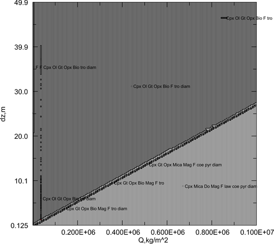
Figure 2:
Phase relations (plotted with PSSECT) within the column as a function of the
time integrated basal flux Q, as explained in the introduction Q scales
linearly with time, such that 1 kg/m2 ~ 1 year. Because of the low
K-content of the column and the large flux increments used in the model,
biotite and is formed throughout the column after the first flux increment
passes through the column. Thereafter a carbonation front advances linearly
upward behind which the stable mineralogy is magnesite (Mag) + coesite + lawsonite (law) + clinopyroxene (Cpx) + dolomite
(Do) + Mica + pyrite. The mineral proportions behind the carbonation front at
the base of the column (Figure 3)
vary because the basal sulfur-flux converts oxidized iron to pyrite at a slower
rate than the carbon-flux converts silicate to carbonate. For the chosen conditions,
all oxidized iron in the rock is converted to pyrite when the pyrite mode
reaches 0.7 vol %, in contrast the amount of pyrite
formed at the carbonation front is 0.4 vol % with
minor amounts of iron present in Cpx, Mag, Mica, and
Do. The column of anomalous phase relations at Q = 40000 kg/m2 is caused by the
failure (indicated by a red field at DZ = ~0.2 m) of an optimization on the
carbonation front.
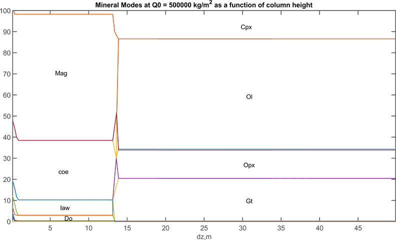
Figure 3: Modal
variations through the metasomatic column at Q = 500000 kg/m2. Obtained using
WERAMI (mode 3, property 25 [modes of all phases => cumulative modes]) and
plotted in MATLAB with the perple_x_simple_plot
script. Because WERAMI does not output the zero-coordinate for cumulative modal
data, the details of the phase relations across the carbonation front are
intentionally confused in the plot (i.e., because I was too lazy to work them
out), this confusion can be resolved by using WERAMI (mode 1) to evaluate the modes
interactively or by plotting the modes obtained using WERAMI (mode 3, property
25 [modes of all phases]) and answering no to the cumulative mode prompt.
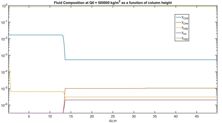
Figure 4: Fluid
composition (species mole fractions) through the metasomatic column at Q =
500000 kg/m2. Obtained using WERAMI (mode 3, property 40 [lagged or
back-calculated fluid chemistry, although the calculation was done without
aqueous chemistry choosing this property provides a shortcut for obtaining the
molecular speciation of the fluid, the more tedious alternative would be to use
property 8 [composition of a solution phase]). The result suggests that for the
subduction scenario without electrolytic species considered in the FRAC2D example, essentially all the molecular
carbon and sulfur released by slab devolatilization would be consumed by mantle
metasomatism within a few meters of the slab
interface.