Perple_X Equilibrium Reactive Transport
Calculations: FRAC2D Model Configuration
Contents
Thoughts on
configuring/running a FRAC2D calculation
Explanation/Definition of Variables
Computation/Plotting of Mass Fluxes
Figures:
Figure 1: FRAC2D vs TITRATE
reactive transport models
Figure 2: Elemental fluxes across
the slab-mantle interface
Figure 4: Total solute-, CH4-,
and CO2-content of the fluid
Figure 5: Bulk column sulfur
content
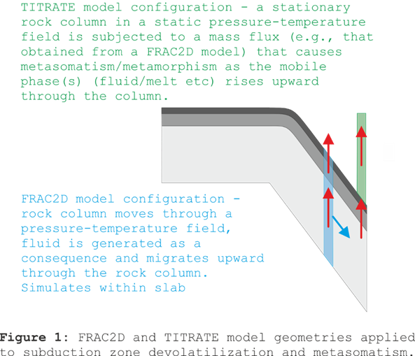
Perple_X is configured to do two general types of
equilibrium reactive transport models, FRAC2D
and TITRATE (Figure 1). Both
configurations are referred to within Perple_X
as 2d-phase fractionation models (Connolly 2005).
In these calculations a 1-dimensional column of rock is subject to
perturbations that lead to the formation of one or more mobile phases (e.g.,
melt and low-density electrolytic or molecular fluids). The rate at which the
perturbations are applied adds a second effective dimension, time, to the
model. The mobile phase(s), i.e., fractionated phase, moves upward through the
column until it is consumed or passes through the top of the column. The two
types of calculations are distinguished by the mechanism for perturbing the
initial equilibrium condition: in FRAC2D calculations, the perturbation is
caused by changing pressure-temperature conditions, as occurs within a
subducted slab or during regional metamorphism; in TITRATE calculations the
perturbation is a mass flux (e.g., the presumed composition of a mobile phase)
to the base of the column, as occurs in the mantle wedge during subduction and
other metasomatic processes. This page documents the FRAC2D configuration,
refer to the TITRATE page for an outline of
TITRATE configuration. FRAC2D and TITRATE represent limiting cases, the
intermediate case in which the column moves through a dynamic P-T field and is
simultaneously subject to a basal mass flux can be computed as a variant of the
FRAC2D configuration in which the TITRATE variable (see below for definition of all input/output
variables) is set.
The
input files for the FRAC2D example outlined here are at www.perplex.ethz.ch/perplex/examples/FRAC2D
are designated by the project name frac2d.
The fractionated, or mobile phase, is represented by the solution model
COH-Fluid+, a model for low-density C-O-H-S fluids. Depending on the aq_lagged_speciation option specified in the Perple_X option file, COH-Fluid+ may represent
either molecular or electrolytic fluids (Connolly and
Galvez, 2018). The example here uses the molecular version of the model and
thus corresponds to an up-date of the subduction model used by Connolly (2005). It is
advisable to work with the molecular model before attempting the electrolytic
model which introduces additional complexity and uncertainty. As in all Perple_X calculations, the project name has no
special significance, the name frac2d used here is chosen solely for purpose of
the example. In this example, equilibrium phase relations are computed for a
column of rock representing the lithologies of the
upper 24.5 km of an oceanic slab as it is subducted incrementally from 80 to
200 km depth, the column is oriented vertically because it is assumed this is
the direction of fluid flow. Consequently, the height of the column is 24.5 km
/ cosine (45 degrees) ~ 34.6 km (see Fig 6 of Connolly 2005),
where 45 degrees is the model slab dip. For purposes of the calculation, the
column is discretized as a set of representative nodes. After each depth
increment, beginning from the lowest representative node, equilibrium phase
relations are computed. If the mobile phase is stable, its mass is removed
(fractionated) from the node and added to the overlying node. The procedure is
then repeated for the overlying node until, ultimately, the top of the column
has been reached. This model carries strong assumptions about the nature of
fluid generation and flow. Specifically, these assumptions are that fluid
generation proceeds from the base of the column upwards, that fluid flow is
instantaneous on the subduction time scale (DT0) and that the flow is pervasive and vertical. There is little
basis for the first assumption, although the case can be made that any fluid
accumulation at depth will induce hydro-mechanical instabilities that causes
the fluid at depth to catch-up fluid at shallower depths (Connolly 1997). Experiments with
alternative assumptions, e.g., that fluid generation proceeds from the top
downward, show that this assumption does not have profound consequences for
mass transport. Pervasive flow maximizes the efficacy of mass transport through
the slab and is therefore a useful extremal scenario. The alternative extremal
scenario, that fluid flow is perfectly channelized by fractures or tube-like
porosity waves (Connolly & Podladchikov, 2007, 2013; Connolly 2010)
corresponds to simple Rayleigh fractionation (e.g., Section 4.4 of Connolly &
Galvez 2018) and is not considered further here. The independent variables
for the calculation the depth of the slab/mantle interface (Z0) and the vertical height above the
base of the slab column (DZ), the
pressure-temperature field from a geodynamic model is expressed as a function
of Z0 and DZ (see below, also Fig 7 of Connolly 2005).
The model neglects the small effect of the divergence in the mass flux on
density and, for the purposes of relating pressure and depth, assumes a
constant density throughout the column and overlying rocks.
The
primary input file for the calculation, frac2d.dat,
is generated using BUILD, by choosing computational mode 7 (2-d Phase
fractionation). In contrast to most Perple_X
calculations in the case of FRAC2D calculations, this input file specifies only
the data sources, thermodynamic components, and solution models to be
considered during the calculation. A second auxiliary file, frac2d.aux, specifies the column lithologies, the model geometry, and the data necessary to
define the pressure-temperature field during subduction. The auxiliary input
file is generated manually, the primary purpose of this document is to explain
the data in the frac2d.aux example so that it can be used as a template for new
calculations.
Files at www.perplex.ethz.ch/perplex/examples/FRAC2D:
frac2d_noaq.dat - the primary input file
(Figure 3).
frac2d_noaq.aux - the auxiliary input file
(Figure 3).
frac2d_noaq_perplex_option.dat - the run time option file (Figure 3).
frac2d_aq.dat - variant with
lagged-aqueous speciation enabled (Figures 2 and 4), the primary input file.
frac2d_aq.aux - variant with
lagged-aqueous speciation enabled (Figures 2 and 4), the auxiliary input file.
frac2d_aq_perplex_option.dat - variant with lagged-aqueous speciation
enabled (Figures 2 and 4), the run time option file.
solution_model.dat - the solution model file.
DEW13HP622ver_elements.dat - the thermodynamic data file.
NOTES: 1) The DEW13 aqueous solute data-base was not converted to
Perple_X format using the default options
specified in the DEW spreadsheet,
it is used here only for purposes of demonstration, the DEW17 aqueous solute
data-base should be used for quantitative applications. 2) These
files can only be read by 6.8.6+ versions of Perple_X.
Steps in a
FRAC2D calculation:
A)
Run BUILD to create the primary input file, e.g., frac2d.dat.
B)
Create the auxiliary input file, e.g., frac2d.aux.
C)
Run VERTEX, answer yes to the fractionate phases prompt and fractionate the
mobile phases of interest (e.g., COH-Fluid+).
D)
Plot and/or analyze phase relations using PSSECT and WERAMI (see section 3, Figures 2, 3, 4). Note that in fractionation
calculations, the data reported by VERTEX include the amount and composition of
the mobile phase prior to fractionation. In FRAC2D calculations, the amount of
the mobile present at a given height within the column is the product of the
mobile phase generated at that height plus any mass gained by fractionation of
the mobile phase at greater depths.
Thoughts on
configuring/running a FRAC2D calculation:
E)
If you are unfamiliar with Perple_X, familiarize yourself
with the programs by following a tutorial such as www.perplex.ethz.ch/perplex_66_seismic_velocity.html.
F) Set
auto_refine to off or manual, using the
low-resolution (exploratory stage) result will identify problems quickly, these
problems must be resolved before a high-resolution (auto-refine stage) result
is attempted.
G)
Before configuring your own calculation, begin at step C, above, using the
input files at www.perplex.ethz.ch/perplex/examples/frac2d. Verify that you are
able to obtain, understand, and analyze the output generated by the example.
H)
Increase complexity gradually: Do not begin with an electrolytic
multi-component fluid, rather begin with water, add molecular volatiles, and
lastly add solutes. Do not begin with complex lithologic
chemistry, rather begin with elements in a single oxidation state and exclude
minor and/or poorly constrained elements. Construct phase diagram sections for
each lithology within your model rock column over the entire
pressure-temperature range of interest. If the phase relations in these
sections do not make sense, then the phase relations in a FRAC2D calculation
certainly will not make sense.
Explanation/Definition of FRAC2D
Variables
Variables
used to describe the FRAC2D calculation, unless otherwise indicated these are
specified in the frac2d.aux file or
computed on output:
AREA - the cross-sectional area of the subducted
rock column, AREA = MASS/ZBOX/RHO.
ANNEAL - if .true., then at the initial condition of the
calculation: a) if fluid is stable at any node in the column, it is removed and
the composition of the node adjusted accordingly; b) the representative masses
(MASS) of all nodes are renormalized
to 1 kg.
C - the number of thermodynamic components
specified in frac2d.dat
CLAY_1_1 ... CLAY_1_C
... ... ...
CLAY_N_1 ... CLAY_N_C
- the molar compositions of the N
column lithologies, from the base of the column
upward. The components in the composition must be entered in the same order as
the components are entered in frac2d.dat.
For calculations in which the fluid is electrolytic it is advisable to use
elemental components. See www.perplex.ethz.ch/perplex/faq/oxide_to_elemental_component
conversion.pdf for an illustration of the oxide-to-elemental conversion used
for the frac2d example. Note that these compositions are extensive. If ANNEAL is .true.,
the mass of the composition will be automatically adjusted to 1 kg. If ANNEAL is .false.,
the molar mass of each layer composition should be comparable.
C_1_0 ... C_1_NORD
... ... ...
C_NPOLY_0... C_NPOLY_NORD
- the coefficients of the NPOLY NORD'th order
polynomials that define the within slab geotherms,
such that T(K) on the N'th
geotherm is T_N = sum(C_N_I*ZI, I =
0,...,NORD). NOTE: Perple_X
does (cannot) not test that the polynomials are valid, therefore it is
advisable to plot the geotherms over the entire depth
range relevant to a calculation. In some cases it may be impossible to
represent a geotherm with a single polynomial, when this is the case use the PZFUNC option to specify the geotherms or explicit P(Z0,DZ)-T(Z0,DZ)
functions.
DIP - slab dip in degrees
DPDZ - the pressure gradient with depth (bar/m).
DPDZ = RHO(kg/m3)*g(m2/s)*(1 bar/105 Pascal), where g is gravitational acceleration (10 m/s2)
and RHO is the average density of
the column and any overlying rock. Perple_X
can be modified to compute a thermodynamically consistent pressure for a loaded
self-gravitating column; such complications seem unwarranted in light of other
sources of uncertainty.
DT0 - the time interval (s) corresponding to
one depth increment of the column, DT0
= DZ0/cosine(DIP)/V_SUB
DYNAMIC - if .true. Pressure and temperature
are a function of the Z0-DZ coordinate. If DYNAMIC is .false., pressure and
temperature are solely a function of DZ.
DZ - height above the base of the column; as
DZ = 0 at Z0, DZ is negative
within the column (see ZBOX).
DZ0 - the incremental change in depth of the
column during subduction, DZ0 = (Z0MIN-Z0MAX)/NINT
DZGEO_1...DZGEO_NPOLY - the
within slab (orthogonal) depths of the NPOLY
geotherms that define the within slab P-T field.
MASS - the mass (g) associated with a
representative node within the column. If ANNEAL
is true, MASS is automatically
adjusted to 1 kg; otherwise MASS is
the mass corresponding to the extensive molar composition of the layer
composition (CLAY_I_J, J = 1...C).
MASS_I - the mass (g) of a component
transported by mobile phase I (e.g.,
fluid and/or melt).
NINT - the number of depth increments as the
column is subducted from Z0MIN to Z0MAX. NINT = 1d_path_nodes -
1, where 1d_path_nodes is specified in frac2d_perplex_option.dat.
NORD - the order of the polynomials used to
describe the within slab P-T field.
NPOLY - the number of geotherms
used to describe the within slab P-T field, three should be adequate for most
purposes. The within column temperature is computed by fitting an (NPOLY-1)'th
order polynomial to the geotherms (see Connolly 2005).
RHO - the average density (kg/m3) of
the column and overlying rock (see DPDZ),
RHO = DPDZ/g*(105
Pa/bar)
P - pressure (bar) at any point within the
column, P = Z*DPDZ.
Q - the flux (g/m2-s) of a
component transported by mobile phase I
through the column over time interval DT0
(e.g., fluid or melt) Q = MASS_I/AREA/DT0 (see step D below).
QINT - the time-integrated flux (g/m2)
transported through the column by mobile phase I (see step D below).
PZFUNC - if .true., then internal
functions are used to compute the P-T field of the column, e.g., from
analytical functions (Davies, GJI, 1999) or tabulated results from, e.g., a
geodynamic model. This option requires that the user program the functions.
T - temperature (K).
TITRATE - if .true., then the column is
subject to a basal mass flux.
VERBOS - if .true., then VERTEX
prints the amount and composition of the mobile phase at each node to the
console. Additionally, if ANNEAL is also .true., then
VERTEX outputs the initial composition at each node and the average composition
of each layer after annealing.
V_SUB - the subduction rate (m/s).
V_HOR - the horizontal component of the slab
velocity (m/s), V_HOR = V_SUB*cosine(DIP).
Z - the absolute depth (m) of any point
within the column, as DZ increases upward, Z
= Z0-DZ.
ZBOX - the vertical unit of discretization for
the column in meters, i.e., the rock column is composed of boxes with a
vertical dimension of ZBOX. The
representative nodes of the column are located at DZ_I = -ZTOT+ZBOX*(1/2+[I-1]); thus the representative nodes at the top and bottom of the
column are at DZ_TOP = -ZBOX/2 and DZ_BOT = -ZTOT+ZBOX/2, respectively. NOTE:
the nodal coordinates of a layer should be entered in WERAMI or PSSECT to
compute fluxes, e.g., to compute the flux across the top of the column, compute
properties at column depth -ZBOX/2.
ZLAY_1...ZLAY_N - the vertical thicknesses (m)
of the N lithological layers within
the column, numbered from the base of the column upward. The vertical thickness
is equal to the thickness of the layer orthogonal to the slab interface divided
by the Cosine of the slab dip (DIP).
NOTE that the layers are discretized with a resolution ZBOX, thus the layer
thicknesses should be an integer multiple of ZBOX. If this is not true, then the model layer thickness will be (ZLAY_I\ZBOX)*ZBOX, where \ denotes the integer quotient. When a computation is
run in VERTEX, the actual layer thicknesses and the nodal coordinates of the
top and bottom of each layer are output to the console.
ZSURF - value of the depth coordinate at the
surface (m), used for the computation of pressure at depth, i.e., P(bar) = (Z0-DZ)*DPDZ.
ZTOT - the total vertical thickness of column
(m), ZTOT = sum(ZLAY_I, I = 1...N).
Z0 - depth (m) at the top of the column (m),
i.e., the depth of the slab/wedge interface.
Z0MIN - the initial depth (m) of the slab/mantle
interface
Z0MAX - the final depth (m) of the slab/mantle
interface
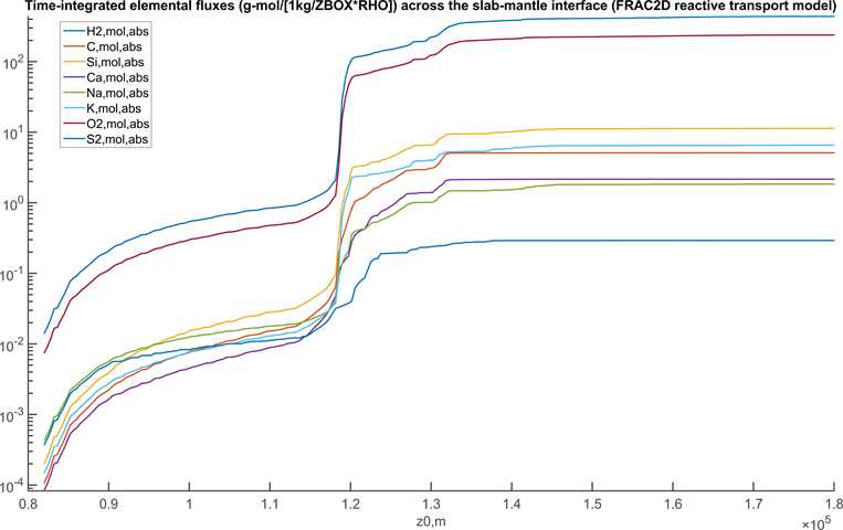
Figure 2:
Time-integrated elemental fluxes across the slab-mantle interface. The
negligible fluxes of Fe, Al, and Mg are not shown. NOTES: 1) the fluxes must be scaled
by ZBOX and RHO (see variable definitions above)
to obtain rational units (e.g., g-mol/m2);
2) the option file linked from this page disables electrolytic fluid speciation
so that carbon, sulfur, hydrogen, and oxygen are the only mobile elements. To
reproduce the figure presented here the aq_lagged_speciation
option must be set to T (true).
Computation and Plotting of Mass Fluxes
A)
Set the absolute option to T in frac2d_perplex_option.dat.
B)
Set the cumulative option to T in frac2d_perplex_option.dat if cumulative fluxes are desired,
otherwise the fluxes are instantaneous, i.e., the average flux over the time
interval DT0.
C)
After setting the above options, start WERAMI:
i) Select
operation mode 3 (properties a long a 1d path).
ii) Construct a linear profile, from (Z0
= Z0MIN, DZ = -ZBOX/2) to (Z0 = Z0MAX, DZ = -ZBOX/2).
iii) For optimal resolution specify NINT + 1 points for the profile.
iv) Select property 36 (all phase and/or system
properties).
v) Specify option 2 (properties of a phase).
vi) Specify the name of the fractionated
phase, e.g., COH-Fluid+.
vii) Answer y or n to the Include fluid in ... properties prompt,
the answer is irrelevant for present purposes.
iix) The output is
in the indicated tab file, e.g., frac2d_1.tab.
ix) Exit.
D) Plot the amount of the
component of interest (e.g., S2_g) using perple_x_simple_plot
(MATLAB), PSTABLE, or PYWERAMI. If the cumulative option is F or default, the plotted quantity
corresponds to the MASS_I (g) of the component that is transported by the fluid
across the slab/mantle interface (at DZ+ZBOX/2 = 0) as the top of the column is
subducted from depth Z0 to Z0+DZ0.
The instantaneous flux, i.e., the flux averaged over the time interval DT0, Q (g/m2-s) = MASS_I/AREA/DT0. If the cumulative option is T, then the plotted quantity is the cumulative mass TOT_MASS_I of the component transported
by the mobile phase, the time-integrated mass flux QINT (g/m2) is TOT_MASS_I/AREA. The data in the tab file can be
edited in a spreadsheet program so that Q
and/or QINT are output directly.
Alternatively, the axes of the plot may be rescaled to indicate the appropriate
flux.
E)
If a calculation is done with more than one mobile phase (e.g., melt and
low-density fluid), step C must be repeated for each phase and the results
summed to obtain the total mass flux transported by the mobile phases.
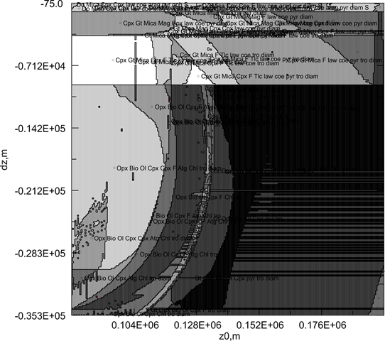
Figure 3: Phase relations within the subducted column as
a function of column depth (Z0) and height within the column (DZ) plotted with
PSSECT. Irregularities occur because small oscillations in the bulk composition
at the representative nodes caused by metasomatism affect the stability of
minor phases. These oscillations can be dampened by increasing NINT and decreasing
ZBOX. The example shown here is for a calculation in which the fluid is
solute-free (aq_lagged_speciation = F). Phase relations plotted directly with
PSSECT for solute-bearing systems are often illegible, in such cases phase
boundaries should be located by tabulating the modal abundances of the stable
phase (WERAMI, mode 2, property choices 7, 25, or 36) and a plotting
script (e.g., MATLAB or PYWERAMI).
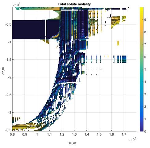
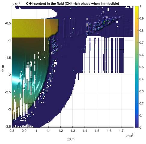
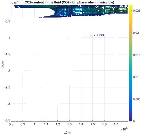
Figure 4:
Total solute molality and CH4- and CO2-content (mole fraction) in the fluid
phase. Where no data is plotted the fluid is not stable. The data for this figure
was generated with WERAMI (mode 2), property choice 40, and plotted in MATLAB
with the perple_x_simple_plot script. The plot of
methane concentration gives a false impression of the importance of such fluids
in this example, i.e., the amount of the methane-rich fluid is minor.
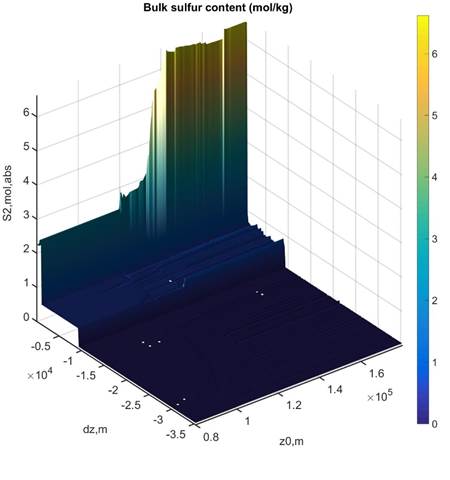
Figure 5:
Bulk
sulfur content in the column. The pattern suggests that sulfur is scoured from
the fluid as it infiltrates into progressively more silicic lithologies
toward the slab surface. The three-dimensional perspective obscures the result
that the maximum sulfur content is realized at the base of the sedimentary
layer and that it subsequently decreases almost to the original sedimentary
sulfur content at the slab interface. The data for this figure was generated
with WERAMI (mode 2), property choice 6 (or 36) and plotted in MATLAB with the perple_x_simple_plot script.