NOTE:
this page is out-of-date because the option keywords referred to here
(indicated in red) are modified or obsolete
in 6.8.6+ versions of Perple_X, the page is
nonetheless useful if the relation of the current options (indicated
in blue) to the former options is understood:
iteration
keyword - values
i1 and
i2, i1
is now (6.8.4+) specified by the resolution_factor
keyword and i2 is
specified by the refinement_points keyword.
initial_resolution
- prior to 6.8.6, initial resolution took one value that specified the static
compositional resolution for the exploratory stage of an auto-refine
calculation. The static compositional resolution during the auto-refine stage
was then computed as initial_resolution/auto_refine_factor_I.
In 6.8.6 initial_resolution
takes two values, v1
and v2,
that correspond to the static compositional resolution during the exploratory
and auto-refine stages of an auto-refine calculation. Thus, where the text below
refers to a value of auto_refine_factor_I
the same effect in the current version of Perple_X
is obtained by setting v2 =
v1/auto_refine_factor_I.
i.e., increasing auto_refine_factor_I had
the same affect as decreasing the v2.
A
brief discussion of adaptive minimization keyword group for the current (6.8.6)
version of
Perple_X is at Perple_X_why_it_often_does_not_work.
The precision and
accuracy of phase diagram section and phase fractionation calculations in
Perple_X hinges on two groups of runtime
keywords specified in the perplex_option.dat file. The adaptive minimization keyword
group (iteration, initial_resolution, final_resolution, auto_refine_factor_I,
reach_increment, global_reach_increment, solvus_tolerance and solvus_tolerance_II) determines the accuracy and
precision with which Perple_X computes
phase relations at an individual grid point in a phase diagram section. The grid
parameters keyword group (grid_levels, x_nodes, y_nodes, 1d_path, and
linear_model) determines the number of grid points used to map the phase
relations of a phase diagram section. This page is concerned only with the first
group. The relevant grid parameters used in the examples presented here, have been chosen to obviate the mapping of phase
relations as a prominent source of error. The first
example discussed here primarily illustrates of the role of the final_resolution
keyword, while the second example illustrates the role
of reach_increment, auto_refine_factor_I, and solvus_tolerance_II
keywords in resolving problems related to the spurious and stepped solvi that
may appear in
Perple_X calculations involving non-ideal
solution models.
The challenge in using
Perple_X effectively is to find keyword
values that produce a high quality result at minimal computational cost. In
brief, the keywords have the following roles (refer to perplex_options.html for
more detailed descriptions):
initial_resolution
- is the initial (molar) compositional resolution during the exploratory stage
(see auto-refine) of a calculation. Decreasing the value of this keyword always
improves the quality of a calculation, but is particularly expensive in terms of
memory. The diagnostic **error ver041**
during the exploratory stage of a calculation indicates initial_resolution is
too fine. Typically a value between 1e-1 and 5e-2 is feasible, small changes in
this value have large influence on memory requirements.
auto_refine_factor_I
- initial_resolution/auto_refine_factor_I is the
effective initial resolution
during the final (auto-refine) stage of a calculation. This keyword permits
finer effective initial resolution during the auto-refine stage than would be
possible in the exploratory stage due to memory limitations. Increasing the
value of this keyword always improves the quality of a calculation. The
diagnostic **error ver041** during the
auto-refine stage of a calculation indicates auto_refine_factor_I is too large.
Typically a value between 2 and 8 is feasible. Calculations with the same
initial_resolution to auto_refine_factor_I ratio should yield essentially
identical results.
final_resolution -
is the final (molar) compositional resolution. During adaptive minimization,
compositions are iteratively refined until their precision is better than the
specified value of final_resolution. The final_resolution does not affect memory
usage, but because it controls the number of iterations it may have a strong
influence on the amount of time required for calculations, particularly for
calculations with multicomponent solution phases. Small values of final_resolution
may cause numerical instability, the diagnostic **warning
ver042** indicates this condition (e.g., Fig
2c). Until this threshold is reached,
decreasing final_resolution always improves the quality of computational
results. As a
rule of thumb, on 32-bit machines, numerical stability becomes problematic
if final_resolution <10-4
mol.
iteration - this
keyword takes two values, i1 and i2,
the default values for this keyword are probably optimal. i1
is the factor by which compositional precision increases in each iteration, the
lowest value permitted for i1 is two, increasing i1
from this value decreases the amount of time required for adaptive minimization
(Connolly 2009), but increases memory consumption (diagnostic **error
ver058**). i2 controls Perple_X's
ability to distinguish stable phases from nearly stable phases and is the number
of (perceived) metastable phases considered during adaptive minimization. As a
consequence i2 has a strong influence on the accuracy of phase
relations in close proximity to phase boundaries. Experience suggests that
increasing i2 beyond its default (4) yields little if any
improvement to computational results, while decreasing this value does not have
major benefits in terms of computational resources.
solvus_tolerance
- this keyword specifies the
minimum distance (in
normalized composition
space) between two compositions of a solution phase at which the compositions
are considered to represent distinct (immiscible) phases of the solution.
Compositions that are separated by a distance less than solvus_tolerance
are considered to represent a single phase whose composition is computed as the
weighted average of the different compositions of the solution. For reasons
discussed below, the default value for this tolerance is much larger than the
theoretical resolution of the adaptive minimization algorithm. The effect of
this parameter is cosmetic.
solvus_tolerance_II
- this keyword specifies a parameter that is used as a criterion for
selecting the metastable phase compositions that are to be refined during adaptive minimization. This parameter can be
adjusted to eliminate stepped solvus boundaries along
which the compositions of the immiscible phases of a solution change by
increments more closely related to the effective initial_resolution
than the requested final resolution for the
calculation. This keyword is discussed in greater detail at perplex_options.html,
see also Example 2 below.
reach_increment
(and/or global_reach_increment)
- this keyword can be used to force Perple_X to widen the interval
over which the estimated composition of a phase may change between successive iterations during adaptive minimization.
This parameter can be adjusted to eliminate spurious solvi
that may occur in calculations than involve solution models that predict immiscibility.
This keyword is discussed in greater detail
below.
Example
1: Pelite
Model, Effect of final_resolution, auto_refine_factor_II and reach_increment
The phase diagram
sections below illustrate the effect of changing the final_resolution, auto_refine_factor_II
and reach_increment keywords on the calculation of phase relations
involving immiscible feldspar phases. Unless otherwise indicated the adaptive
minimization keyword group have their default values, the grid
parameters keyword group values (grid_levels
= 4, x_nodes = y_nodes = 100) are slightly finer than the default. The input files for this
calculation are here.
 Figure
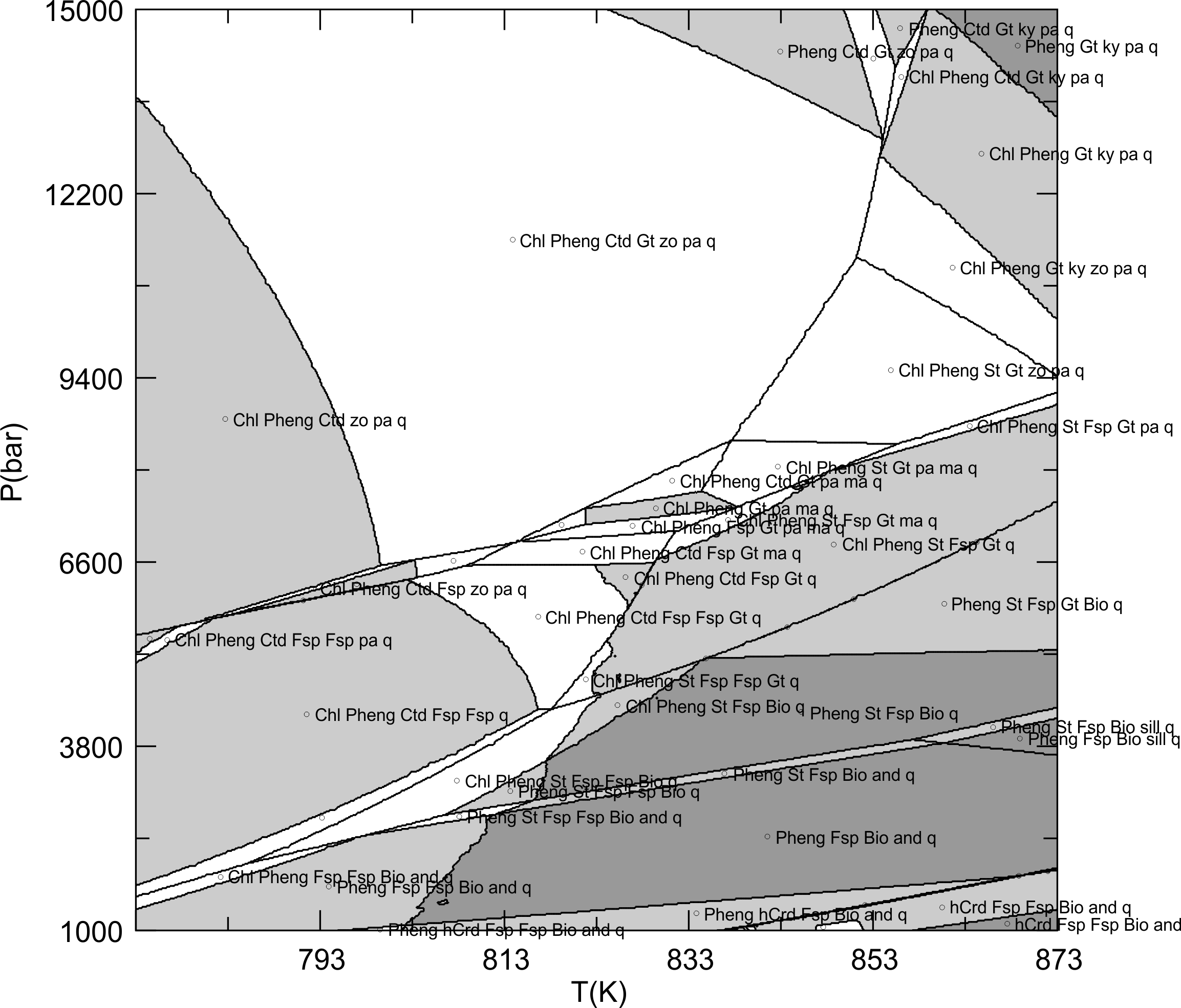
1. The phase diagram section obtained with the default adaptive
minimization keyword values (initial_resolution = 0.067, auto_refine_factor_I
= 2, iteration = [3, 4], solvus_tolerance = auto, solvus_tolerance_II
= 0.25). The phase names have been edited for clarity. Phase relations in this
section are complicated by the existence of a solvus for the feldspar (Fsp)
solution model. This solvus is indicated in the output by the phase fields in
which two (or more) coexisting phases are represented by the same solution model
(e.g., the phase field Chl+Pheng+St+Fsp+Fsp+Bio). The boundaries of the solvus
are recognized by the conditions at which the only one feldspar is stable (e.g.,
the boundary between the Chl+Pheng+St+Fsp+Fsp+Bio and Chl+Pheng+St+Fsp+Bio
phase fields). With the default adaptive minimization keyword settings some of
these phase boundaries are poorly resolved, additionally some spurious solvi are
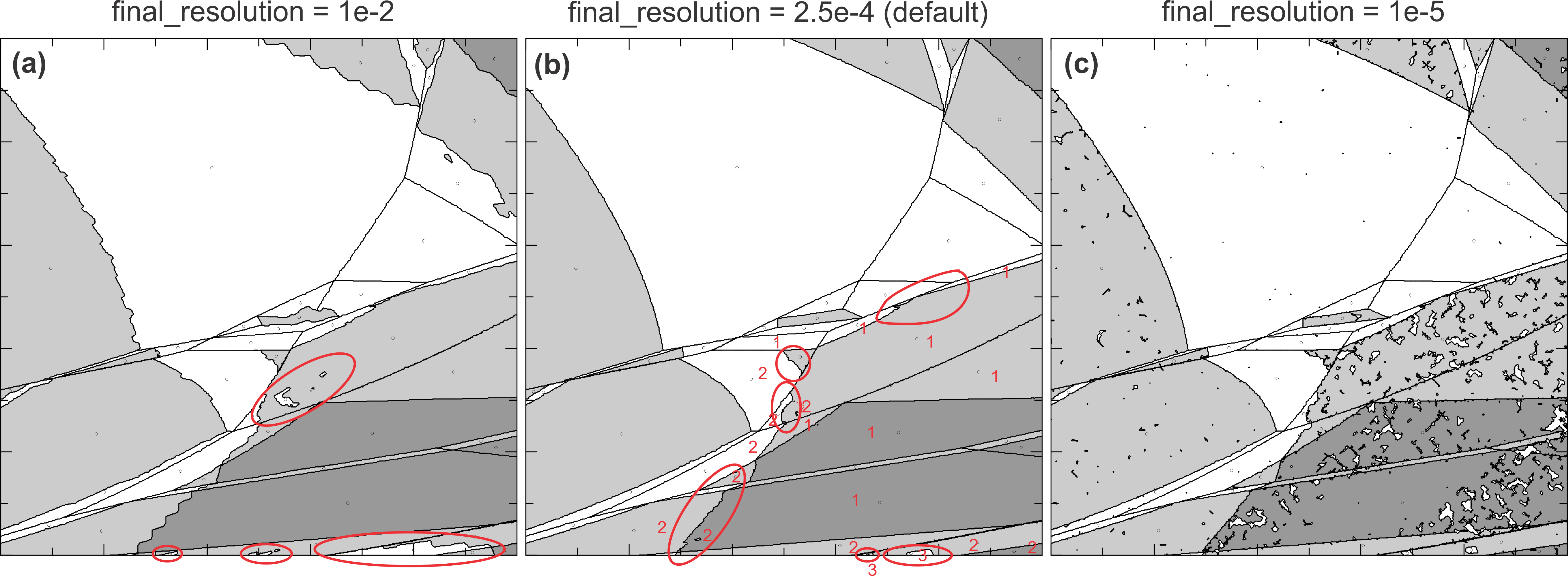
also present (these flaws are circled by red curves in Fig 2b). In Perple_X,
characteristically, spurious solvi have more phases than are stable in the
correct result and are often patchy or have geometries that look unnatural
(e.g., they often form striped patterns). Spurious solvi can also be recognized
by the fact that their location is usually sensitive to computational parameters
such as initial_resolution and final_resolution. Spurious solvi
can always be eliminated by increasing the value of the solvus_tolerance
keyword, however this approach to eliminating the solvi hides rather than solves
the underlying problem. Moreover using large values of the solvus_tolerance
keyword increase the probability that truly immiscible phase compositions will
be homogenized.
Figure
2. [Below]. Results obtained with inadequate (a), default (b),
and excessive (c) values of the final_resolution keyword (in b numbers
indicate the number of feldspar phases stable in each field), text labels have
been suppressed for clarity. Inadequate final_resolution leads to irregular
phase boundaries and spurious solvi. With the default final_resolution (b)
the extent of spurious solvi is reduced and all non-solvus phase boundaries are
well resolved. In (c) excessive final_resolution has caused numeric
instability manifest by irregular white patches where the adapative minimization
algorithm has failed to converge (these patches can be distinguished from
spurious solvi from the indicated phase assemblage, e.g., if Perple_X
does not converge, WERAMI will indicate that there is no data at the relevant
conditions).

The calculations
illustrated in Fig 2 indicate that the default value of the final_resolution
keyword is appropriate for the calculation. The fact that the prominent flaws in
Fig 2b are associated with a solvus boundary indicates that these flaws are
related to difficulties in converging to the correct compositions of the
immiscible solution. These
difficulties arise in Perple_X because the
adaptive minimization algorithm assumes that if phase compositions have been discretized with
resolution
dn, then the accuracy
for any compositional variable xn is ±dn.
Therefore during iterative refinement the compositional estimate is not allowed
to move outside the interval xn±dn,
this has the consequence that if two compositions are in reality miscible, but
separated by a distance > dn,
the compositional estimates cannot converge during iteration. Thus, although
Perple_X usually resolves phase compositions
with accuracy ~final_resolution, in the case of solvi the final
resolution may be limited by the effective initial resolution (i.e.,
initial_resolution/auto_refine_factor_I), hence if solvus_tolerance is set to
automatic, then the value of the tolerance is generously estimated as 3/2*initial_resolution/auto_refine_factor_I.
These considerations suggest two ways of resolving solvus related
problems, the first is to use finer effective initial resolution, and the second
is to widen the interval over which phase compositions are allowed to vary.
Unfortunately, there is no universal solution for these problems, so trial
and error may be necessary to achieve high quality results. From the perspective
of minimizing computational cost, it is less expensive (and only slightly less
accurate) to obtain finer effective initial resolution by increasing
auto_refine_factor_I than it is by reducing the value of initial_resolution. For
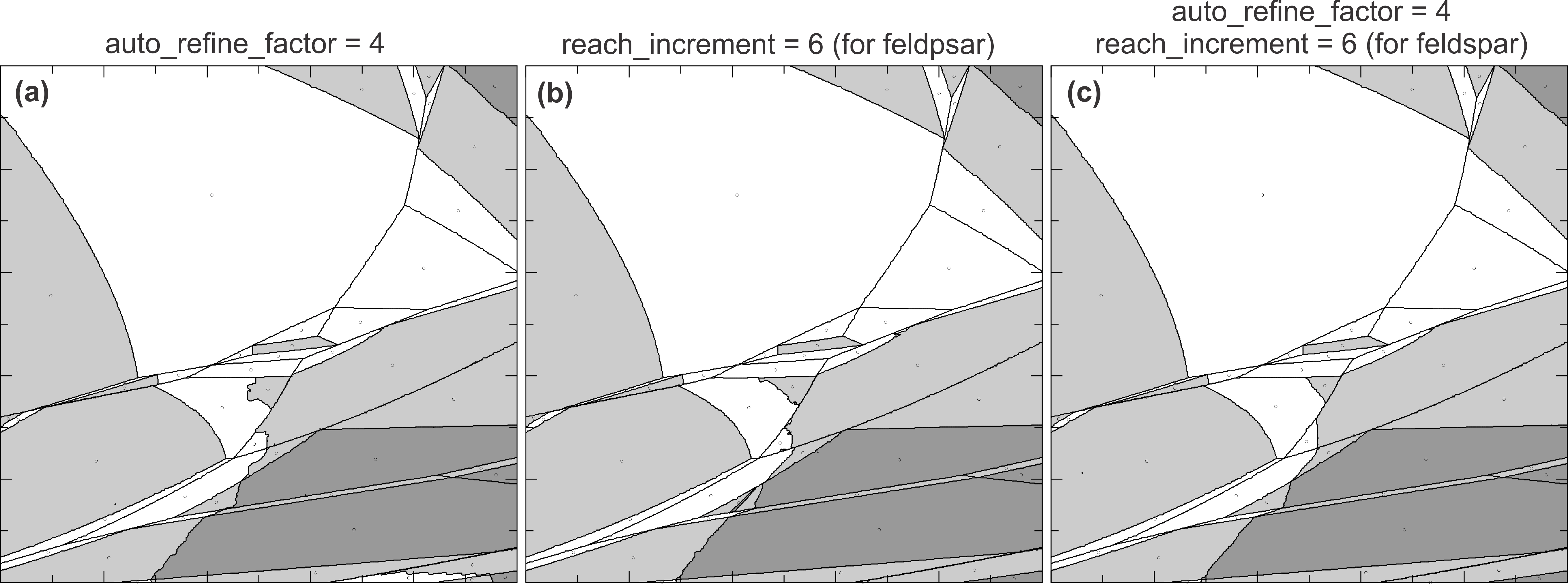
the present example, increasing the effective resolution by doubling
auto_refine_factor (Fig 3a) does little to improve the computational
result. The range over which compositions are allowed to vary during iteration
can be changed for all phases by specifying a non-zero value for the global_reach_increment
keyword, in which case the range is xn±global_reach_increment*dn.
However, for many problems the cost of increasing the range globally is
prohibitive, an inexpensive alternative is to only widen the range of
the solution phase(s) that exhibits immiscibility by specifying a reach_increment
for that solution. A complication in this regard is that the reach_increment
must be specified in the solution model file (e.g., solution_model.dat, Fig
4) rather than the runtime option
file (e.g., perplex_option.dat). For the
present example, applying a reach_increment of 6 to the feldspar solution model eliminates the spurious solvi, but does not completely eliminate rough
solvus boundaries. However, increasing auto_refine_factor_I together with
reach_increment does lead to a good quality result (Fig 3c).
Figure
3. Neither increasing auto_refine_factor_I (a) nor the reach_increment
for the feldspar model (b) in isolation is completely successful in eliminating
the flaws apparent in the calculation depicted in Fig 2a, but applying both
changes in tandem produces a high quality result (c).

begin_model
                           | ternary feldsar (fuhrman & lindsley, am min, 1988)
feldspar
2                          | model type: Margules or Ideal
3                          | 3 endmembers
abh
an
san
0 0 0                      | endmember flags = 0 if the endmember is part of the solution.
0. 1. 0.1   0              | range and resolution for albite, imod = 0 -> cartesian subdivision
0. 1. 0.1   0              | range and resolution for anorthite, imod = 0 -> cartesian subdivision

begin_excess_function
w(abh abh san) 27320.   -10.3  .394
w(abh san san) 18810.   -10.3  .394
w(an  an  san) 52468.      .0   .0
w(an  san san) 47396.      .0  -.12
w(an  an  abh) 28226.      .0   .0
w(an  abh abh) 8471.       .0   .0
w(an  abh san) 100045.5 -10.3 -0.76
end_excess_function

2                          | 2 site (O-site and T-site) entropy model

3 1.                       | 3 species on O-site, 1 site per formula unit.
z(Na) = 1 abh
z(Ca) = 1 an

2 2.                       | 2 species on T-site, 2. sites per formula (al-avoidance model)
z(Al) = 1/2 + 1/2 an

reach_increment 6

end_of_model
|
Figure
4. To widen the range over which the composition of a specific solution
is allowed to vary during adaptive minimization, the reach_increment keyword
must be added to the solution model (e.g., in solution_model.dat) immediately
before the end_model keyword, as illustrated here (and highlighted in red) for
the feldspar model (NOTE: there is no equals
sign between a keyword and its value).
Example
2: Spurious and Stepped Solvi: the Effect of reach_increment and
solvus_tolerance_II
The phase diagram
sections below illustrate the effect of changing the reach_increment, auto_refine_factor_II,
and solvus_tolerance_II keywords on the calculation of phase relations
involving immiscible clinopyroxene phases represented by the Omph(GHP)
solution model. Unless otherwise indicated the adaptive
minimization keyword group have their default values, the grid
parameters keyword group values (grid_levels
= 4, x_nodes = y_nodes = 40) lead to somewhat coarser mapping of the phase
relations than illustrated in the previous example. The input files for this
calculation are here.
 Figure
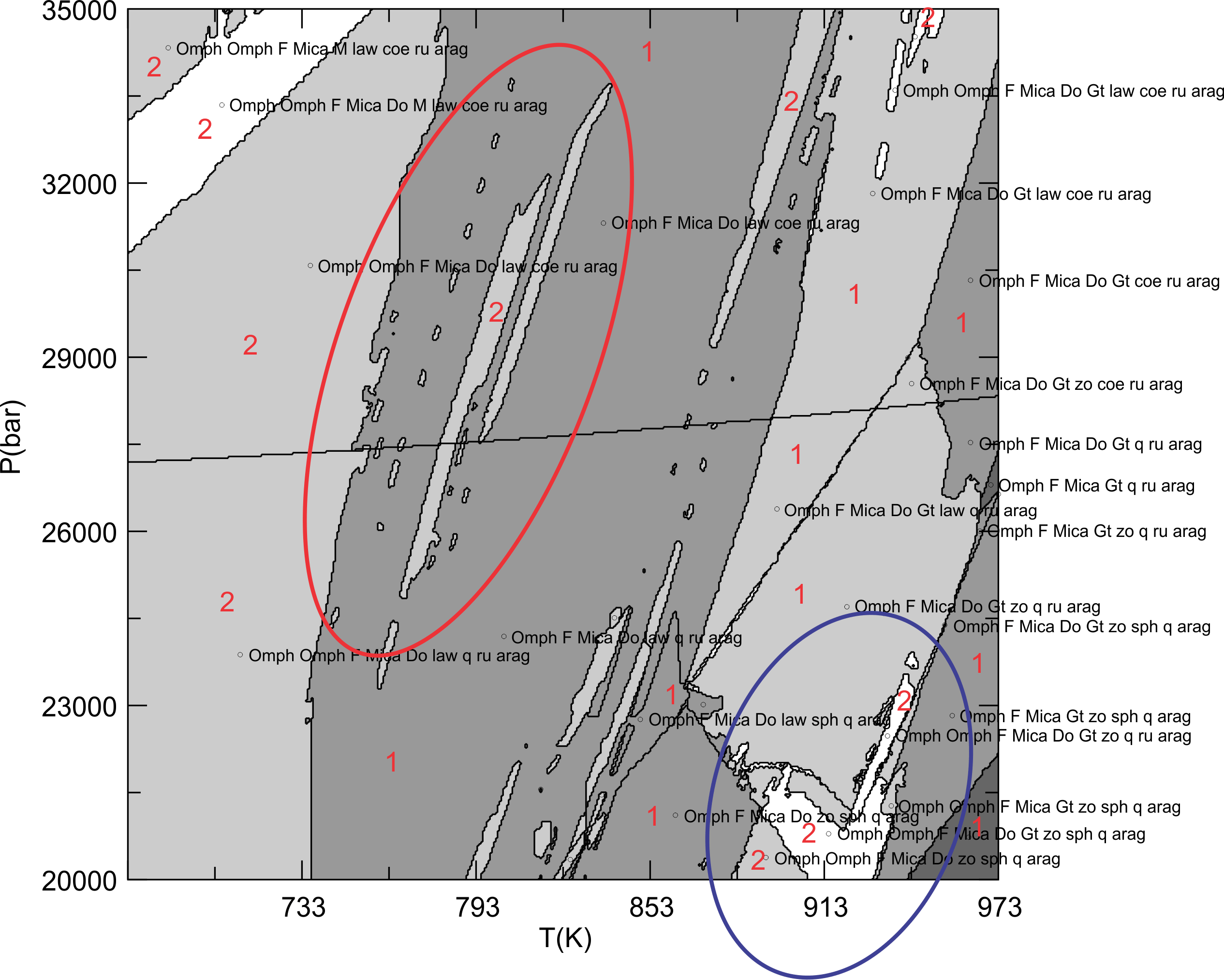
5. The phase diagram section obtained with the default adaptive
minimization keyword values (initial_resolution = 0.067, auto_refine_factor_I
= 2, iteration = [3, 4], solvus_tolerance = auto, solvus_tolerance_II
= 0.25). The phase names have been edited for clarity. Phase relations in this
section are complicated by immiscibility predicted by the clinopyroxene (Omph)
solution model. The immiscibility is manifest in the Perple_X
calculation by both real and spurious solvi (solvi are phase fields in which
two, or more, coexisting phases are represented by the same solution model,
e.g., Omph+Omph+F+Mica+Do+zo+sph+q+arag). The red
numerals indicate the number of stable phases in each phase field that
correspond to the clinopyroxene model. In Perple_X,
characteristically, spurious solvi have more phases than are stable in the
correct result and are often patchy or have geometries that look unnatural
(e.g., they often form striped patterns, e.g., within the area circled in
red). Spurious solvi can also be recognized
by the fact that their location is usually sensitive to computational parameters
such as initial_resolution and final_resolution. In addition to
the spurious solvi, this calculation also illustrates a second problem referred
to here as a "stepped" solvus (circled in blue). In Perple_X,
characteristically, stepped solvi are recognized by highly irregular (though
often periodic) boundaries, these irregularities correspond to conditions at
which one of the immiscible phases abruptly changes composition. Fig
6 illustrates
how the reach_increment parameter can be used to eliminate the spurious solvi,
while Fig 7
illustrates how solvus_tolerance_II can be manipulated to eliminate the stepped
solvus. Spurious solvi
can always be eliminated by increasing the value of the solvus_tolerance
keyword, however this approach to eliminating the solvi hides rather than solves
the underlying problem. Moreover using large values of the solvus_tolerance
keyword increase the probability that truly immiscible phase compositions will
be homogenized.
Spurious solvi arise in Perple_X because the
adaptive minimization algorithm assumes that if phase compositions have been discretized with
resolution
dn, then the accuracy
for any compositional variable xn is ±dn.
(where the subscript n indicates the values in the nth
iteration of an adaptive minimization). During iterative refinement the compositional estimate is not allowed
to move outside the interval xn±dn-1,
this has the consequence that if two compositions are in reality miscible, but
separated by a distance > dn,
the compositional estimates cannot converge during iteration. Thus, although
Perple_X usually resolves phase compositions
with accuracy ~final_resolution, in the case of solvi the final
resolution may be limited by the effective initial resolution (i.e.,
initial_resolution/auto_refine_factor_I). For this reason, if solvus_tolerance is set to
automatic (as recommended), then the value of the tolerance is generously estimated as
3/2*initial_resolution/auto_refine_factor_I.
These considerations suggest two ways of eliminating spurious solvi (aside from hiding them by increasing solvus_tolerance), the first is to use finer effective initial resolution, and the second
is to widen the interval over which phase compositions are allowed to vary. In
general the default settings in the runtime
option file are such that the effective initial resolution cannot be
increased significantly (see Fig 3a),
accordingly here the range over which compositions are allowed to vary during iteration
is changed. This range
can be changed for all phases by specifying a non-zero value for the global_reach_increment
keyword, in which case the range is xn±global_reach_increment*dn.
However, for many problems the cost of increasing the range globally is
prohibitive, an inexpensive alternative is to widen the range of only the solution
phase(s) that exhibits immiscibility by specifying a reach_increment
for that solution. A minor complication in this regard is that reach_increment
must be specified in the solution model file (e.g., solution_model.dat,
Fig 4) rather than the
runtime option file (e.g., perplex_option.dat). For the
present example, applying a reach_increment of six to the clinopyroxene solution model eliminates the
spurious solvi (Fig 6)
that were initially present (Fig 5).
Even
with a reach_increment of six the calculated section retains a number of flaws,
these include some wavy or irregular phase boundaries (circled in
red
in Fig 6),
the stepped solvus (circled in blue), and
the seemingly univariant boundary between sphene-bearing assemblages at low
pressure and rutile-bearing assemblages at high pressure (circled in
green).
The univariant rutile-sphene boundary is plausible topologically, but improbable
because it implies that the corresponding reaction does not effect the
composition of omphacite as it evidently does at higher temperature where the
transition corresponds to a narrow divariant field that extends to the (stepped)
omphacite solvus which then degenerates back to a univariant boundary. There is
no universal rule that governs the course of action to be taken to
eliminate/resolve these flaws, but my personal guiding principal is to maximize
both the initial and final resolution (in this regard I remark that there is no
reason to use the high mapping resolution specified by the grid
parameters keyword group for this problem, thus if the time required by
high compositional resolution is a concern, this concern can be alleviated by
using much lower mapping resolution). In the present case, finer final_resolution
is not an option because values below 2e-4 cause numerical instabilities (warning
ver042), the effective initial
resolution can be improved by either reducing initial_resolution
or increasing auto_refine_factor_I. Here I
opt for the latter as it is generally more efficient, and after some
experimentation find that I can increase auto_refine_factor_I to at least 17.5
(corresponding to an effective initial resolution of 0.0038 mol) before VERTEX
runs out of memory (error ver041). The result of
this high resolution calculation (Fig 7a)
is satisfying in that the sphene-rutile boundary (circled in
green)
is now adequately resolved, but the stepped solvus (circled in
blue)
persists and small spurious solvi (circled in red)
have reappeared. The spurious solvi are eliminated by increasing the
reach_increment for the Omph(GHP) model to eight (Fig
7b), but because the stepped solvus is extremely narrow in composition
(~0.03 mol) eliminating this flaw by further increases in initial resolution is
prohibitively expensive. A less expensive alternative course of action is to
reduce solvus_tolerance_II. The disadvantage
of adjusting solvus_tolerance_II is that while it improves the resolution of
solvus boundaries, it may degrade the quality of normal phase boundaries. Thus,
reducing solvus_tolerance_II to 0.1 mol (Fig
7c) and still further to 0.05 mol (Fig 7d)
improve the resolution of the solvus, but introduce minor flaws (circled in
red)
that were not present in the initial version of the high resolution calculation
(Fig 7b).
Figure
6. Increasing the reach_increment specified for the clinopyroxene model,
Omph(GHP), ultimately eliminates the spurious solvi evident in Fig
5. Increasing reach_increment always
improves the accuracy of computational results, but the cosmetic quality of the
section (i.e., how the section appears rather than the information embodied
within it) does not necessarily improve until the reach_increment is
sufficiently large to completely eliminate all spurious solvi. Increasing
reach_increment also influences the stepped solvus (circled in
blue in Fig
5) because the increased range
permitted for the clinopyroxene composition allows Perple_X
greater freedom to adjust the phase compositions during iteration; however the
shape of the solvus is clearly unnatural.

Figure
7. Stepped solvi and solvus_tolerance_II.

 Figure
1. The phase diagram section obtained with the default adaptive
minimization keyword values (initial_resolution = 0.067, auto_refine_factor_I
= 2, iteration = [3, 4], solvus_tolerance = auto, solvus_tolerance_II
= 0.25). The phase names have been edited for clarity. Phase relations in this
section are complicated by the existence of a solvus for the feldspar (Fsp)
solution model. This solvus is indicated in the output by the phase fields in
which two (or more) coexisting phases are represented by the same solution model
(e.g., the phase field Chl+Pheng+St+Fsp+Fsp+Bio). The boundaries of the solvus
are recognized by the conditions at which the only one feldspar is stable (e.g.,
the boundary between the Chl+Pheng+St+Fsp+Fsp+Bio and Chl+Pheng+St+Fsp+Bio
phase fields). With the default adaptive minimization keyword settings some of
these phase boundaries are poorly resolved, additionally some spurious solvi are
also present (these flaws are circled by red curves in Fig 2b). In Perple_X,
characteristically, spurious solvi have more phases than are stable in the
correct result and are often patchy or have geometries that look unnatural
(e.g., they often form striped patterns). Spurious solvi can also be recognized
by the fact that their location is usually sensitive to computational parameters
such as initial_resolution and final_resolution. Spurious solvi
can always be eliminated by increasing the value of the solvus_tolerance
keyword, however this approach to eliminating the solvi hides rather than solves
the underlying problem. Moreover using large values of the solvus_tolerance
keyword increase the probability that truly immiscible phase compositions will
be homogenized.