Running BUILD: problem setup
Running VERTEX: phase diagram section computation
Running PSSECT: phase diagram section depiction
Running WERAMI: extraction of phase abundances
Running PSVDRAW: plot of phase abundances
Figures:
Figure 1: Phase relations for a Martian model aerotherm and composition
Figure 2: Phase abundances for a Martian model aerotherm and composition
There are several ways in which Perple_X '07 can be used to extract properties along a 1-dimensional path such as a geotherm (or, in the case of Mars an "aerotherm"), if the path coordinates are known in advance these include:
1) Construction of a 1-dimensional phase diagram section in which the physical conditions are defined as a monotonic polynomial function of a path variable (in the case of a geotherm P=f(T) or T=f(P)).
2) Construction of 2-dimensional phase diagram section with VERTEX, which is then sampled along the path with WERAMI.
3) Construction of a 1-dimensional phase diagram section in which the path is defined by a list of coordinates that need not be monotonic (e.g., a circular P-T path).
Additionally, any of these methods can be applied to a path which is defined by an isopleth (e.g., an adiabat or conditions for which the abundance, composition or any other bulk or phase property is constant) that is recovered from an initial 2-dimensional calculation (see properties along a contour).
Of the methods listed above the first is always preferable in terms of efficiency and accuracy. An example of method 1 is given in the Perple_X '06 tutorial on phase fractionation tutorial. Method 2 may be useful if a large number of paths are required for a single bulk composition or simply that the necessary 2-dimensional calculation has already been done (an example of this method is given in the archaic Perple_X '06 phase diagram section tutorial). This page provides a briefly documented example of the Perple_X-user dialogs necessary for method 3. Method 3 is useful when the path of interest is too complex to be described by a simple polynomial and is essential in cases where the path coordinates are not monotonic (e.g., a P-T path that passes through a maximum in either pressure or temperature).
The disadvantages of Method 3 are that the resolution of the calculation is limited by the number of coordinates specified (i.e., there is no automatic refinement of phase boundaries) and that the output generated by PSSECT depicts phase relations (Figure 1) as function of nodal coordinates (i.e., the position of coordinate in the input list). The latter limitation results because the PSSECT expects regularly spaced plotting coordinates, however because the path is 1-dimensional data recovered from WERAMI can be used, as illustrated here, to construct a 2-dimensional modal variation diagram that is effectively a 1-dimensional phase diagram (Figure 2).
The calculation illustrated here is for the mineralogy of the Martian mantle for pressures from 1-24.5 GPa (in fact, because the aerotherm is monotonic, method 1 would be preferable in this case, but method 3 is used for the sake of illustration). In contrast to "tutorials" (which are essentially non-existent for Perple_X '07) little attempt is made to document the dialogs provided below, inexperienced users are referred to the seismic velocity tutorial and the build prompt and Perple_X option file pages for additional explanation.
In the following dialogs the Perple_X prompts are in normal font, user responses are in bold font and explanatory comments are written in red.
c\jamie\Berple_X>build
NO is the default ([cr]) answer to all Y/N prompts (help)
Enter name of problem definition file to be created, <100 characters, left justified [default = in]: (help)
in24.dat
Enter thermodynamic data file name, left justified, [default = hp02ver.dat]: (help)
The sfo05ver.dat data base, which is primarily from Stixrude & Lithgow-Bertelloni (2005, Khan et al. 2006), can be used over the entire range of mantle conditions, but is for a simplistic chemical model (see also example #23). Stixrude & Lithgow-Bertelloni (2007) published a more comprehensive data base that is formatted for Perple_X in the file stx07ver.dat.
sfo05ver.dat
The first major block of prompts from BUILD determine the manner in which the chemical components defined within the thermodynamic data file are to be used. VERTEX permits components to be treated in four different ways: saturated phase components are components whose chemical potentials are determined by the (assumed) stability of a phase, most commonly a fluid, containing these components; saturated components are components whose chemical potentials are determined by the (assumed) stability of a phase(s) containing only the saturated-phase and saturated components; mobile components are components whose chemical potentials are defined explicitly; and thermodynamic components are components whose chemical potentials are the dependent variables of a phase diagram calculation. Phase diagram calculations require the specification of at least one thermodynamic component.
The current data base components are:
MGO AL2O3 SIO2 CAO FEO
Transform them (Y/N)? (help)
n
Calculations with a saturated phase (Y/N)? (help)
The phase is: FLUID
Its compositional variable is: Y(CO2), X(O), etc.
n
Calculations with saturated components (Y/N)? (help)
n
Use chemical potentials, activities or fugacities as independent variables (Y/N)? (help)
n
Select thermodynamic components from the set: (help)
MGO AL2O3 SIO2 CAO FEO
Enter names, left justified, 1 per line, [cr] to finish:
MGO
AL2O3
SIO2
CAO
FEO
The second major block of prompts defines the explicit variables for the phase diagram calculation.
Specify computational mode: (help)
1 - Unconstrained minimization
2 - Constrained minimization on a grid [default]
3 - Constrained minimization on a 1d grid
4 - Output pseudocompound data
5 - Phase fractionation calculations
Unconstrained optimization should be used for the calculation of composition, mixed variable, and Schreinemakers diagrams. Gridded minimization can be used to construct one- and two-dimensional phase diagram sections.
3
Enter path
coordinates from a file (Y/N)?
y
In this mode
VERTEX/WERAMI read path coordinates from a file, the file must be formatted so
that the coordinates of each point are on a separate line, the coordinates are,
in order: P(bar) T(K)
The data base has P(bars) and T(K) as default independent potentials. Make one dependent on the other, e.g., as along a geothermal gradient (y/n)? (help)
n
Enter the coordinate file name, < 100 characters, left justified [default = coor.dat]:
aerotherm.dat
File: aerotherm.dat
Does not exist, you must create it before running VERTEX.
Specify component amounts by weight (Y/N)?
y
Enter weight amounts of the components: (help)
SIO2 TIO2 AL2O3 FEO MGO CAO NA2O K2O H2O CO2
for the bulk composition of interest:
31.5 2.31 42.71 2.49 18.71
The next prompts define the output required by the user.
Do you want a print file (Y/N)?
Enter the plot file name, <100 characters, left justified [default = pl]: (help)
pl24
The final block of prompts from BUILD define the phases for the calculation.
Exclude phases (Y/N)? (help)
y
Here, experience leads me to make exclude stishovite (stv) as the sfo05ver.dat data base seems to overestimate its stability.
Do you want to be prompted for phases (Y/N)?
n
Enter names, left justified, 1 per line, [cr] to finish:
stv
Do you want to treat solution phases (Y/N)?
y
Enter solution model file name [default = solut_07.dat] left justified, <100 characters: (help)
solut_07.dat
...diagnostics omitted...
BUILD reads the solution model file and determines which solutions are consistent with the problem as specified by the user. The diagnostics (omitted here) can usually be ignored. They are useful if you discover that a solution you wish to include is not present in the list of solutions BUILD offers.
Select phases from the following list, enter 1 per line, left justified, [cr] to finish: (help)
Omph(GHP)
O(SG) E(SG)
Omph(HP) GaHcSp O(HP)
Cpx(l) Cpx(h)
Sp(JR) Sp(GS) Sp(HP)
GrPyAlSp(B
GrPyAlSp(G Gt(HP) Gt(EWHP)
Gt(WPH) Qpx
Mn-Opx
Wus(fab) Aki(fab) Pv(fab)
Ppv(og) O(stx) Wad(stx)
Ring(stx) Sp(stx) Gt(stx)
C2/c(stx) Opx(stx) Cpx(stx)
Cpx(stx7) cOmph(HP) CrGt
CrOpx(HP) Opx(HP) Cpx(HP)
CrSp Wus(stx7)
Aki(stx7) Pv(stx7) O(stx7)
Wad(stx7)
Ring(stx7) Sp(stx7)
Wus(fab)
Pv(fab)
O(stx)
Wad(stx)
Ring(stx)
C2/c(stx)
Opx(stx)
Cpx(stx)
Sp(stx)
Gt(stx)
Aki(fab)
Enter calculation title:
Martian SNC model
As indicated by after the path coordinate file prompt in BUILD, the file containing the list of coordinates for the path must be created before VERTEX can be run to calculate the phase equilibrium. As noted in association with the prompt this file must consist of a list of coordinates, the coordinates of each point must be on separate lines. The file used for the calculation described here is aerotherm.dat.
The calculation dialog depicted here is done with the "auto_refine" option set to "on" be sure to verify this setting in your version of perplex_option.dat or copy the version used here to your working directory.
c\jamie\Berple_X> vertex
VERTEX begins by echoing the current settings for computational options, these are either the default internal values or values specified in the file perplex_option.dat.
Perple_X options
are currently set as:
Keyword:
Value: Permitted values [default]:
dependent_potentials off
off [on ]
bad_number
0. [0.0]
solvus_tolerance 0.050
0->1 [0.05], 0 => p=c pseudocompounds, 1 => homogenize
zero_mode
0.1E-05 0->1 [1e-6], < 0 => off
zero_bulk
0.1E-05 0->1 [1e-6], < 0 => off
adaptive optimization
iteration limit
4 >0 [3], value 1 of iteration
keyword
refinement factor 3
>2*r [5], value 2 of iteration keyword
refinement points 10
0->100 [10], value 3 of iteration keyword
initial_resolution 0.10
0->1 [0.1], 0 => off
stretch_factor
0.016 >0 [0.0164]
reach_factor
0.9 >0.5 [0.9]
subdivision_override off
[off] lin str
auto_refine
aut off [manual] auto
auto_refine_factor_I 3
>=1 [3]
auto_refine_factor_II 5
>=1 [10]
auto_refine_factor_III 2
>=1 [3]
auto_refine_slop 0.010
[0.01]
hard_limits
off [off] on
Gridded minimization parameters:
x_nodes
20 / 60 [20/40], >0, <2048; effective x-resolution 20/ 473
nodes
y_nodes
20 / 60 [20/40], >0, <2048; effective y-resolution 20/ 473
nodes
grid_levels
1 / 4 [1/4], >0, <10
1d_path
10 /150 [20/150], >0, <2048
Parameters for Schreinemakers and Mixed-variable diagram
calculations:
variance
1 /99 [1/99], >0, maximum true variance
increment
0.100 /0.025 [0.1/0.025], default search/trace variable increment
efficiency
3 [3] >0 < 6
reaction_format min
[min] full stoichiometry S+V everything
reaction_list
off [off] on
console_messages on
[on] off
short_print_file on
[on] off
WERAMI/MEEMUM output options:
compositions
mol wt [mol]
proportions
vol wt [vol] mol
interpolation
on off [on ]
extrapolation
off on [off]
vrh_weighting
0.5 0->1 [0.5]
cumulative_modes
off [off] on
Worst case (Cartesian) compositional resolution (mol %)
Stage Adaptive
Non-Adaptive* Non-Adaptive**
Exploratory 0.146
10.000 10.000
Auto-refine 0.049
2.000 5.000
* - composition/mixed variable diagrams, ** - Schreinemakers diagrams
To change these options edit or create the file perplex_option.dat
See:
www.perplex.ethz.ch/perplex_options.html
VERTEX then requests the problem definition file created by BUILD (in24.dat):
Enter problem definition file name (i.e. the file created with BUILD), left justified:
in24.dat
and lists the input/output files to be used/created for the calculation. Several additional output files are created in addition to the plot file pl24 requested by the user, among these are: bpl24 named by adding the prefix "b" to the plot file name, pseudocompound_glossary.dat, and auto_refine_in24.dat.txt. These files contain information about the range of compositions considered in the calculation. It is only essential to be aware of these files if you wish to store or analyze results in a different directory than the working directory for VERTEX, in which case the files must be copied to the relevant directory.
Reading
thermodynamic data from file: sfo05ver.dat
Writing print output to file: none requested
Writing plot output to file: pl24
Writing pseudocompound glossary to file: pseudocompound_glossary.dat
Reading solution models from file: solut_07.dat
Writing bulk composition plot output to file: bpl24
Total number of pseudocompounds: 588
The following line indicates the beginning of the exploratory stage of the two cycle calculation
** Starting
exploratory computational stage **
Calculations along an arbitrary path with or without fractionation are done by the same internal routines within VERTEX, thus, even if a fractionation calculation has not been specified in BUILD, VERTEX prompts for fractionation.
Fractionate phases (y/n)?
n
After completing the exploratory stage VERTEX outputs the compositional ranges of the stable solution phases, this information is used in the subsequent high resolution calculation.
Endmember
compositional ranges for model: Wus(fab)
Endmember Minimum Maximum
per
0.62498 0.63394
Endmember compositional ranges for model: Aki(fab)
Endmember Minimum Maximum
cor
0.00333 0.00778
aki
0.79333 0.80667
Endmember compositional ranges for model: Pv(fab)
Endmember Minimum Maximum
aperov 0.00556
0.01556
perov 0.81111
0.81556
Endmember compositional ranges for model: O(stx)
Endmember Minimum Maximum
fo
0.73778 0.80000
Endmember compositional ranges for model: Wad(stx)
Endmember Minimum Maximum
wad
0.73111 0.82444
Endmember compositional ranges for model: Ring(stx)
Endmember Minimum Maximum
ring 0.46222
0.72444
Endmember compositional ranges for model: Sp(stx)
Endmember Minimum Maximum
sp
0.31704 0.34667
Endmember compositional ranges for model: Gt(stx)
Endmember Minimum Maximum
gr
0.05333 0.15148
alm
0.10889 0.30667
maj
0.02222 0.74315
Endmember compositional ranges for model: C2/c(stx)
Endmember Minimum Maximum
c2/c 0.74889
0.75778
Endmember compositional ranges for model: Opx(stx)
Endmember Minimum Maximum
en
0.68889 0.76667
fs
0.23333 0.28667
Endmember compositional ranges for model: Cpx(stx)
Endmember Minimum Maximum
di
0.68667 0.89333
hed
0.07556 0.17333
With the exception of the initial header section and prompts the output from VERTEX for the final "auto-refine" stage of the calculation is identical except that the compositional ranges and limits are now modified by information gleaned from the exploratory stage.
Reading data for
auto-refinement from file: auto_refine_in24.dat
2 pseudocompounds generated for: Wus(fab)
4 pseudocompounds generated for: Aki(fab)
4 pseudocompounds generated for: Pv(fab)
3 pseudocompounds generated for: O(stx)
4 pseudocompounds generated for: Wad(stx)
10 pseudocompounds generated for: Ring(stx)
2 pseudocompounds generated for: Sp(stx)
829 pseudocompounds generated for: Gt(stx)
2 pseudocompounds generated for: C2/c(stx)
8 pseudocompounds generated for: Opx(stx)
34 pseudocompounds generated for: Cpx(stx)
Total number of pseudocompounds: 902
** Starting auto_refine computational stage **
Endmember compositional ranges for model: Wus(fab)
Endmember Minimum Maximum
per
0.62623 0.63326
Endmember compositional ranges for model: Aki(fab)
Endmember Minimum Maximum
cor
0.00368 0.00702
aki
0.79470 0.80063
Endmember compositional ranges for model: Pv(fab)
Endmember Minimum Maximum
aperov 0.00474
0.01563
perov 0.81035
0.81669
Endmember compositional ranges for model: O(stx)
Endmember Minimum Maximum
fo
0.73766 0.79949
Endmember compositional ranges for model: Wad(stx)
Endmember Minimum Maximum
wad
0.73131 0.82535
Endmember compositional ranges for model: Ring(stx)
Endmember Minimum Maximum
ring 0.46333
0.72445
Endmember compositional ranges for model: Sp(stx)
Endmember Minimum Maximum
sp
0.31640 0.34657
Endmember compositional ranges for model: Gt(stx)
Endmember Minimum Maximum
gr
0.05386 0.15131
alm
0.10892 0.30603
maj
0.02170 0.74315
Endmember compositional ranges for model: C2/c(stx)
Endmember Minimum Maximum
c2/c 0.74919
0.75747
Endmember compositional ranges for model: Opx(stx)
Endmember Minimum Maximum
en
0.68776 0.76665
fs
0.23282 0.28755
Endmember compositional ranges for model: Cpx(stx)
Endmember Minimum Maximum
di
0.68425 0.89130
hed
0.07608 0.17244
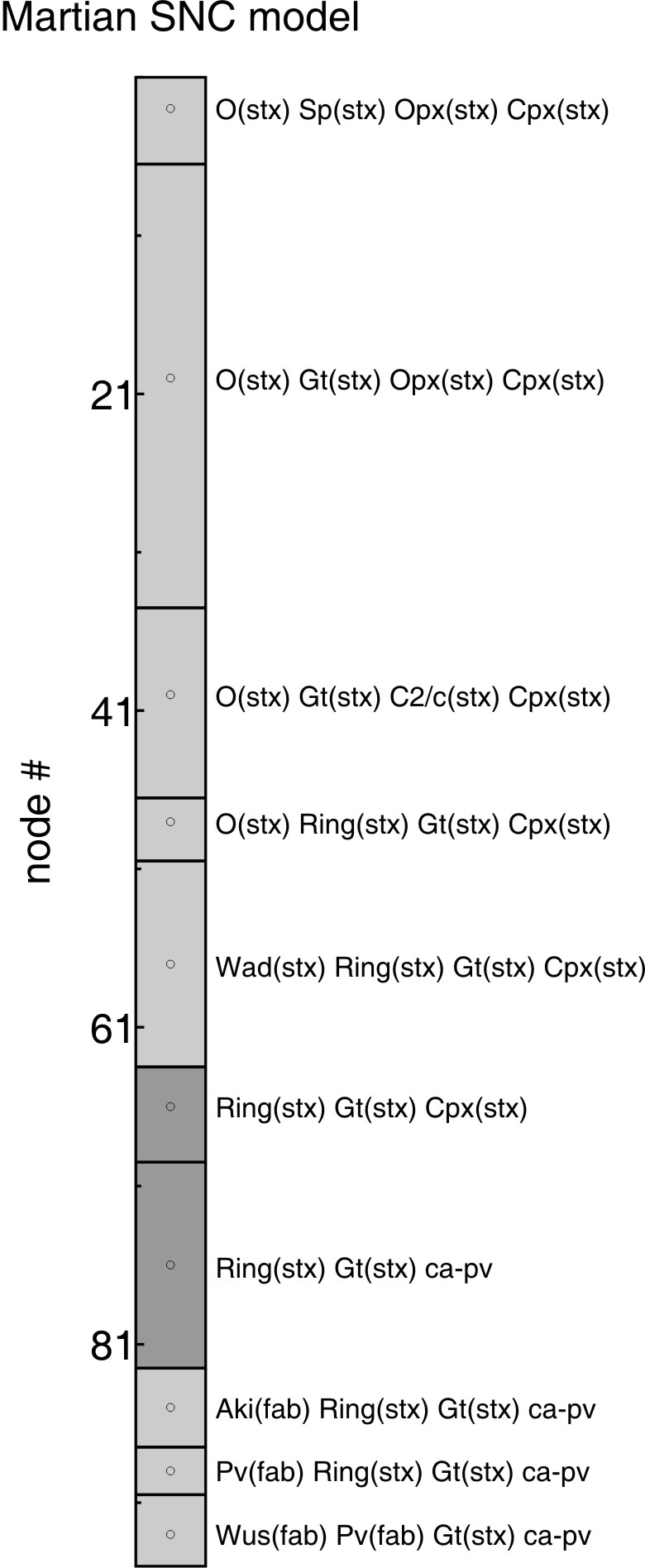
PSSECT generates PostScript graphical output and can be used once the phase diagram section has been calculated with VERTEX. The plot generated by the following dialog with PSSECT shows the computed phase relations in a 1-dimensional section (Figure 1).
c\jamie\Berple_X> pssect
...
Enter problem definition file name (i.e. the file created with BUILD), left justified:
in24.dat
PostScript will be written to file:
pl24.ps
Answer yes to the following prompt to modify features such as axis labeling, size, and shape.
Modify the default plot (y/n)?
y
...
Figure 1. Phase relations (pl24.ps) for a
Martian model composition and aerotherm. The phase relations are plotted as a function of node
#, which corresponds to the position of the physical conditions in the coordinate
file (i.e., aerotherm.dat), e.g., the pressure and
temperature at node 41 is the 41st condition specified in aerotherm.dat (11 GPa,
1898 K, these values can be recovered by using WERAMI in operational mode 1).
WERAMI permits the user to extract information from a phase diagram section at a point, throughout a region, or along a line or curve. The latter two options generate output that can be plotted with programs PSCONTOR, PSVDRAW or PSPTS or imported into general-purpose programs such as Matlab. The dialog and output for each of these modes is detailed in the pseudosection tutorial. Here the second mode is deactivated because of the 1-dimensional character of the output from VERTEX and the third mode is used to extract phase abundances along the model aerotherm.
c\jamie\Berple_X> werami
... information about the option settings omitted here, the only parameter of importance in the present context is the value of the "cumulative_modes" keyword...
Enter problem definition file name (i.e. the file created with BUILD), left justified:
in24.dat
Select operational mode:
1 - compute properties at specified conditions
3 - compute properties along a curve or line (plot with pspts, pt2curv or psvdraw)
0 - EXIT
3
Console output will be echoed in file: rpl24
Writing data to file: cpl24
Enter endpoint 1 for node #
1
Enter endpoint 2 for node #
95
How many points along the profile?
95
Select a property:
1 - Specific enthalpy (J/m3)
2 - Density (kg/m3)
3 - Specific Heat capacity (J/K/m3)
4 - Expansivity (1/K, for volume)
5 - Compressibility (1/bar, for volume)
6 - Weight percent of a component
7 - Mode (Vol %) of a compound or solution
8 - Composition of a solution
9 - Grueneisen thermal ratio
10 - Adiabatic bulk modulus
11 - Shear modulus (bar)
12 - Sound velocity (km/s)
13 - P-wave velocity (Vp, km/s)
14 - S-wave velocity (Vs, km/s)
15 - Vp/Vs
16 - Specific Entropy (J/K/m3)
17 - Entropy (J/K/kg)
18 - Enthalpy (J/kg)
19 - Heat Capacity (J/K/kg)
20 - Specific mass of a phase (kg/m3-solid)
21 - Poisson ratio
22 - Molar Volume (J/bar)
23 - Chemical potentials (J/mol)
24 - Assemblage Index
25 - Modes of all phases
25
For this choice, the perplex_option.dat keyword:
cumulative_modes
influences the output data.
The influence of the cumulative_modes keyword is shown by the plots in Figure 2, this keyword affects only WERAMI output and only property choice #25.
In this mode output is written in two formats:
1 - tabular (spread sheet) format is in file: cpl24
2 - PSVDRAW plot format is in file: scpl24
The x-axis variable for the PSVDRAW plot is: P(bar)
The columns of the tabular form correspond to:
node # P(bar) O(stx) Sp(stx) Opx(stx) Cpx(stx) Gt(stx) C2/c(stx) ...
1.00000 0.00000 56.1998 2.78326 30.0582 10.9587 0.00000 0.00000 ...
2.00000 0.00000 56.2170 2.78692 29.9961 10.9999 0.00000 0.00000 ...
3.00000 0.00000 56.2187 2.80468 29.9353 11.0413 0.00000 0.00000 ...
...
Select operational mode:
1 - compute properties at specified conditions
3 - compute properties along a 1d path (plot with pspts or pt2curv)
4 - as in 3, but input from file
0 - EXIT
0
The datafiles generated by WERAMI for the "modes of all phases" property choice can be imported into spread-sheet programs such as Excel or plotted in the Perple_X program PSVDRAW. The file for the former purpose is cpl24 (prefix "c" + the plot file name), whereas for the latter purpose the file is scpl24 (prefix "sc" + plot file name). The PSVDRAW dialog to generate the plots in Figure 2 is reproduced below.
c\jamie\Berple_X>psvdraw
Enter the Perple_X plot file name:
scpl24
PostScript will be written to file: scpl24.ps
Modify the default plot (y/n)?
y
Modify default drafting options (y/n)?
answer yes to modify:
- picture transformation
- x-y plotting limits
- relative lengths of axes
- text label font size
- line thickness
- curve smoothing
- axes labeling and gridding
y
Modify x-y limits (y/n)?
n
Modify default picture transformation (y/n)?
n
Modify ratio of x to y axis length (y/n)
n
Modify default text scaling (y/n)?
n
Use minimum width lines (y/n)?
n
Fit curves with B-splines (y/n)?
y
Restrict phase fields by variance (y/n)?
answer yes to:
- suppress pseudounivariant curves and/or pseudoinvariant points of
a specified true variance.
n
Restrict phase fields by phase identities (y/n)?
answer yes to:
- show fields that contain a specific assemblage
- show fields that do not contain specified phases
- show fields that contain any of a set of specified phases
n
Modify default equilibrium labeling (y/n)?
answer yes to:
- modify/suppress [pseudo-] univariant curve labels
- suppress [pseudo-] invariant point labels
n
Modify default axes (y/n)?
y
Enter the starting value and interval for major tick marks on
the X-axis (the current values are: 0.125E+05 0.465E+05)
Enter the new values:
0 5e4
Enter the starting value and interval for major tick marks on
the Y-axis (the current values are: 0.00 20.0 )
Enter the new values:
0 20
Cancel half interval tick marks (y/n)?
n
Draw tenth interval tick marks (y/n)?
n
Rescale axes text (y/n)?
n
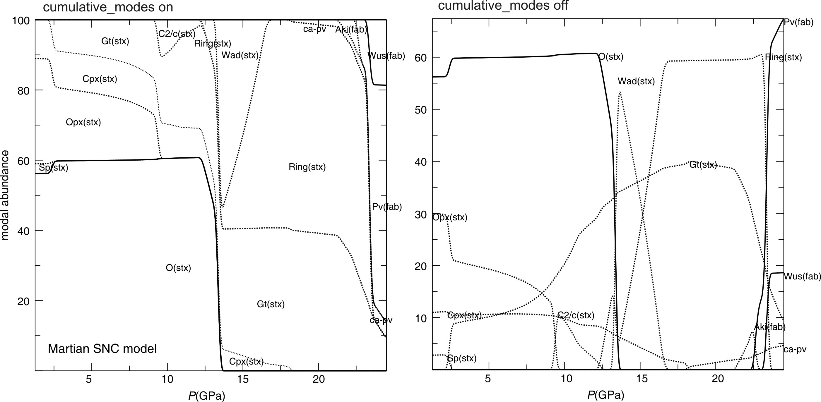
Figure 2. Modal abundances as a function of pressure for a Martian model composition and aerotherm. The left and right plots were obtained with the cumulative_modes keyword set, respectively, to on and off. With cumulative_modes on, the width of each region in the diagram is proportional to the abundance of a phase, in principle it is possible to order the phases so that when cumulative modes are computed the resulting diagram consists of continuous fields. Such ordering is not done by WERAMI with the result that, e.g., the field of Cpx which is continuous from 1 to 18 GPa is represented as two fields with a discontinuity at ~13.7 GPa. Users who wish to obtain continuous fields may consider reordering the columns of the tabular output format generated with cumulative modes set to off to generate obtain a more rational representation.