This page is a map to the Perple_X examples directory. Some of the older examples include explanatory commentary; however, because these examples were prepared decades ago, aspects of the commentary may no longer be relevant. Users should refer to the more recent uncommented plots and dialogs to see how the problem is currently treated. The commentary, such as it is, is progressive, that is to say, things that are explained in the first example are taken for granted in the next. An unfortunate consequence of the out-datedness of the examples is that if calculations are done with current data they no longer illustrate the petrological details initially intended. Despite these problems, the examples provides some idea of how Perple_X can be used. A danger in using the old examples is that the commentary may indicate that some things are not possible when they actually are possible in the current version.
NOTE 1: the problem definition files referred to here were updated on 3/3/08 to function with Perple_X 07. In general the dialogs and plot output have not been updated. To emulate the dialogs for an actual calculation enter solution_model.dat when prompted for the solution model file. If a dialog specifies a thermodynamic data file named hp#ver.dat where # < 02, then enter hp02ver.dat rather than the indicated file name.
NOTE 2: Because this page (as all Perple_X documentation) is usually out-of-date, for most users it may be more useful to browse the perplex/examples folder to find relevant examples and benchmark calculations.
2: Ternary "AFM" diagrams, COH fluid at constrained oxygen fugacity
3: Schreinemakers P-T projection for the system MgO-FeO-Al2O3-KAlO2-SiO2-H2O
6: Silica chemical potential vs. fluid composition Schreinemakers diagram (silicate).
7: Oxygen chemical potential vs. Sulfur chemical potential Schreinemakers diagram (Cu-Fe-Ni)
8: Schreinemakers P-T projection with fluid of variable composition
10: T-X(SiO2) liquidus mixed-variable diagram for the CaO-SiO2 system
11: T-X(O) Screinemakers diagram for a graphite saturated system
13: Phase diagram section at constant bulk composition ("pseudosection") by gridded minimization
16: Solvus calculation for graphite saturated COH fluid by unconstrained minimization
20: Phase relations during adiabatic decompression-induced melting
29: Oxygen fugacity buffer as a function of pressure and temperature
Isobaric T-XCO2 Schreinemakers projection for the SiO2 and fluid saturated system CaO-MgO-Al2O3-SiO2-H2O-CO2.
Commented dialog (dialog1_commented.txt)
Uncommented dialog (dialog1_raw.txt)
Commented print file output (print1_commented.txt)
Commented plot (plot1_commented.gif)
Uncommented plot (plot1.gif)
Problem definition file (in1.dat)
Ternary "AFM" diagrams (projection through feldspar KAlO2 component, not muscovite component KAl3O5 as in the classical Thompson projection, see Example 5) for a system saturated with respect to a COH fluid and graphite at constrained oxygen fugacity.
Commented dialog (dialog2_commented.txt)
Uncommented dialog (dialog2_raw.txt)
Commented print file output (print2_commented.txt)
Commented plot (plot2_commented.gif)
Uncommented plot (plot2.gif)
Problem definition file (in2.dat)
Schreinemakers P-T projection for the water-saturated system MgO-FeO-Al2O3-KAlO2-SiO2, with the additional constraints that: a pure SIO2 phase is stable with all assemblages; the phase that coexists with this SIO2 phase on the SiO2-Al2O3 join (i.e., Ky, Sil, And, Phyl, Dia, Co, Kao, etc.) is stable with all assemblages; the phase that coexists with the above two phases on the KAlO2-Al2O3-SiO2 join (i.e., Kspar, Mu, etc.) is stable with all assemblages.
Commented dialog (dialog3_commented.txt)
Uncommented dialog (dialog3_raw.txt)
Commented print file output (print3_commented.txt)
Commented plots (plot3a_commented.gif, plot3b_commented.gif)
Uncommented plot (plot3.gif)
Problem definition file (in3.dat)
Ternary "AFM" diagrams, similar to example 2, but not graphite saturated. Intended to illustrate the effects of changing the component saturation hierarchy in example 2.
Uncommented dialog (dialog4_raw.txt)
Uncommented plot (plot4.gif)
Problem definition file (in4.dat)
Classical "Thompson AFM diagram" diagrams.
Commented dialog (dialog5_commented.txt)
Uncommented dialog (dialog5_raw.txt)
Uncommented plot (plot5.gif)
Problem definition file (in5.dat)
Silica chemical potential vs. fluid composition Schreinemakers diagram for the system CaO-SiO2-Al2O3-SiO2-H2O-CO2-O2 at constant pressure, temperature, and oxygen chemical potential. An updated on-line version of this example illustrates the conversion of chemical potentials to activities (program MU_2_F).
Commented dialog (dialog6_commented.txt)
Uncommented dialog (dialog6_raw.txt)
Uncommented plot (plot6.gif)
Problem definition file (in6.dat)
Oxygen chemical potential vs. Sulfur chemical potential Schreinemakers diagram for the system Cu-Fe-Ni.
Commented dialog (dialog7_commented.txt)
Uncommented dialog (dialog7_raw.txt)
Uncommented plot (plot7.gif)
Schreinemakers P-T projection for the system CaO-MgO-SiO2-H2O-CO2 with a fluid of variable composition (Connolly & Trommsdorff 1991).
Commented dialog (dialog8_commented.txt)
Uncommented dialog (dialog8_raw.txt)
Uncommented plot (plot8.gif)
Problem definition file (in8.dat)
T-X(Mg)diagram for the system the graphite-saturated system MgO-FeO-Al2O3-K2O-SiO2-C-O-H.
Uncommented dialog (dialog9_raw.txt)
Uncommented dialog for gridded minimization version (dialogj9_raw.txt)
Commented plot (plot9_commented.gif)
Uncommented plot (plot9.gif)
T-X(SiO2) liquidus diagram for the system the CaO-SiO2.
Uncommented dialog (dialog10_raw.txt)
Commented plot (plot10_commented.gif)
Uncommented plot (plot10.gif)
Problem definition file (in10.dat)
T-X(O) Screinemakers diagram for the graphite saturated system CaO-FeO-Al2O3-SiO2-C-O-H-S (Connolly & Cesare 1993, Connolly 1995).
Commented dialog (dialog11_commented.txt)
Uncommented dialog (dialog11_raw.txt)
Commented plot (plot11_commented.gif)
Uncommented plot (plot11.gif)
Problem definition file (in11.dat)
This example is obsolete in Post 06 versions of Perple_X. Mode 1 pseudosection calculation; as documented in the pseudosection tutorial (Connolly & Petrini 2002).
Uncommented dialog (dialog12_raw.txt)
Uncommented plot (plot12.gif)
Problem definition file (in12.dat)
Mode 2 pseudosection calculation. This dialog is for the same problem as Example 12, but illustrates the gridded minimization strategy (Connolly 2005). See alternative versions of examples 7 and 9 (jn7.dat, jn9.dat) for additional examples of gridded minimization.
Uncommented dialog (dialog13_raw.txt)
Uncommented plot (plot13.gif)
Problem definition file (in13.dat)
Molecular fluid speciation as a function of composition with programs SPECIES, PSVDRAW, and COHSRK. Perple_X includes a number or routines for the calculation of the speciation of COHS fluids, this example illustrates the calculation of COHS fluid speciation along the graphite saturation surface as a function of X(O) (the atomic fraction of oxygen relative to hydrogen + oxygen). The same programs can be used to calculate fluid speciation as a function of f(O2) or f(CO2), an example of the dialog for calculation of COHN fluid speciation as a function of f(O2) is also provided below.
Uncommented dialog for COHS as a function of X(O) (dialog15_raw.txt)
Uncommented plots for COHS (plot15.gif)
Uncommented dialog for COHN as a function of f(O2) (dialog15a_raw.txt)
Solvii can be calculated in a number of ways within Perple_X for both solids and fluids, the dialog here illustrates the calculation of the methane- and CO2-rich solvii for COH fluids along the graphite saturation surface as a mixed variable phase diagram computation. To make the diagram two-dimensional the phase relations on the graphite saturation surface are projected onto the H-O join, the position of the solvii in the COH ternary can be computed as illustrated in EXAMPLE 15.
Uncommented dialog (dialog16_raw.txt)
Uncommented plot(plot16.gif)
Problem definition file (in16.dat)
All files (example16.zip)
The same solvii, but calculated by gridded minimization:
Uncommented plot(plotj16.jpg)
Problem definition file (jn16.dat)
Creation of endmembers with FRENDLY for the Holland & Powell (2001, J Pet) and White et al. (2001, JMG) haplo-granite melt models. This method of making endmembers is generally inferior to specifying a "make definition" in the header of thermodynamic file (for example, see the definitions in hp02ver.dat).
Uncommented dialog (dialog17_raw.txt)
Melt fractionation calculation documented in the phase fractionation tutorial.
Problem definition file for the fractionation calculation (in18.dat)
Problem definition file for the pseudosection (ain18.dat)
Uncommented pseudosection showing fractionation path (aplot18.gif)
Mineral modes with and without fractionation along the fractionation path (mplot18.gif)
Phase diagram section depicting melting phase relations as a function of water-content and pressure and temperature along a Barrovian geothermal gradient. This calculation uses gridded minimization and is documented in the T-X, P-X, and X-X pseudosection tutorial as discussed in Connolly (2005). The tutorial describes how to use WERAMI to refine the compositional ranges specified for a solution model.
Problem definition file (in19.dat)
High resolution pseudosection computed for a simplified melt model that excludes the sil8L, fo8L, fa8L, and anL endmembers (high_plot19.gif)
Low resolution pseudosection computed for the full melt model using the in19.dat input file (low_plot19.gif).
Mineral and melt proportions during isentropic decompression by gridded minimization. The calculation is for an ultramafic bulk composition using the pMELTS model of Ghiroso et al (2002) with all remaining data from Holland & Powell (1998). This calculation uses gridded minimization and is documented in the adiabtatic crystallization tutorial as discussed in Connolly (2005).
Problem definition file (in20.dat)
Redrafted and raw pseudosections (plot20_final.gif, plot20_raw.gif)
3D entropy surface (cplot20_3d_entropy.gif)
Two-dimensional (space-time) phase fractionation calculation used to model open system behavior during infiltration-driven subduction zone decarbonation. These input files generate a low resolution version of the example discussed in Connolly (2005). NOTE: The files provided for this example can only be read by pre-6.7.5 versions of Perple_X, current (6.8.6+) versions read the files accessed from the FRAC2D reactive-transport page.
Input files for subduction rate of 0.1 m/y (in21a.dat, in21a.aux)
Input files for subduction rate of 0.02 m/y (in21b.dat, in21b.aux)
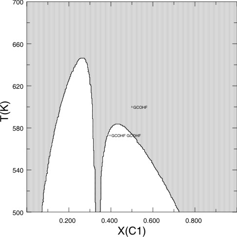
Isobaric H2O-SiO2-Al2O3 saturated phase relations in the KNASH system as a function of Temperature and Composition [X(C2)=K/{K+Na}] by gridded minimization. This example illustrates possible complications from using solvus testing to compute phase relations.
Problem definition file (in22.dat)
Commented graphical output (pl22.gif)
Perplex_option.dat (high initial_resolution and solvus_tolerance) and solut_07.dat files (example22.zip)
Upper mantle mineralogy and seismic velocities. This Perple_X example is provided primarily to demonstrate that even low resolution calculations with Perple_X reproduce results obtained with non-linear optimization strategies.
Comparison of mantle phase relations computed with Perple_X and as computed by Stixrude & Lithgow-Bertelloni [2005, JGR 110, art 2965] (stixrude.pdf)
Computational input file for the calculation (in23.dat). N.b., to reproduce the phase relations as depicted by Stixrude & Lithgow-Bertelloni [2005] with Perple_X it is necessary to exclude stishovite (stv) from the calculation, there is no evident error in the stishovite data, therefore it appears probable that stishovite was also excluded in the published calculation.
Seismic velocity profiles along mantle adiabats across the 660 km transition compared to PREM (mantle_velocity_profiles.pdf). For this calculation, Stixrude & Lithgow-Bertelloni's [2005] data for the upper mantle has been augmented as described in the header of the sfo05ver.dat data file. Mid- to lower- mantle calculations require the solution models Wus(fab), Ppv(og), Pv(fab), and Aki(fab) in solution_model.dat in addition to those specified in in23.dat for the upper mantle calculation.
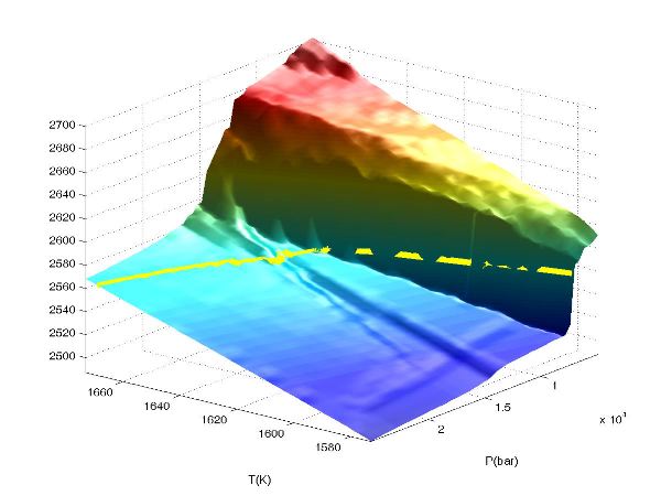
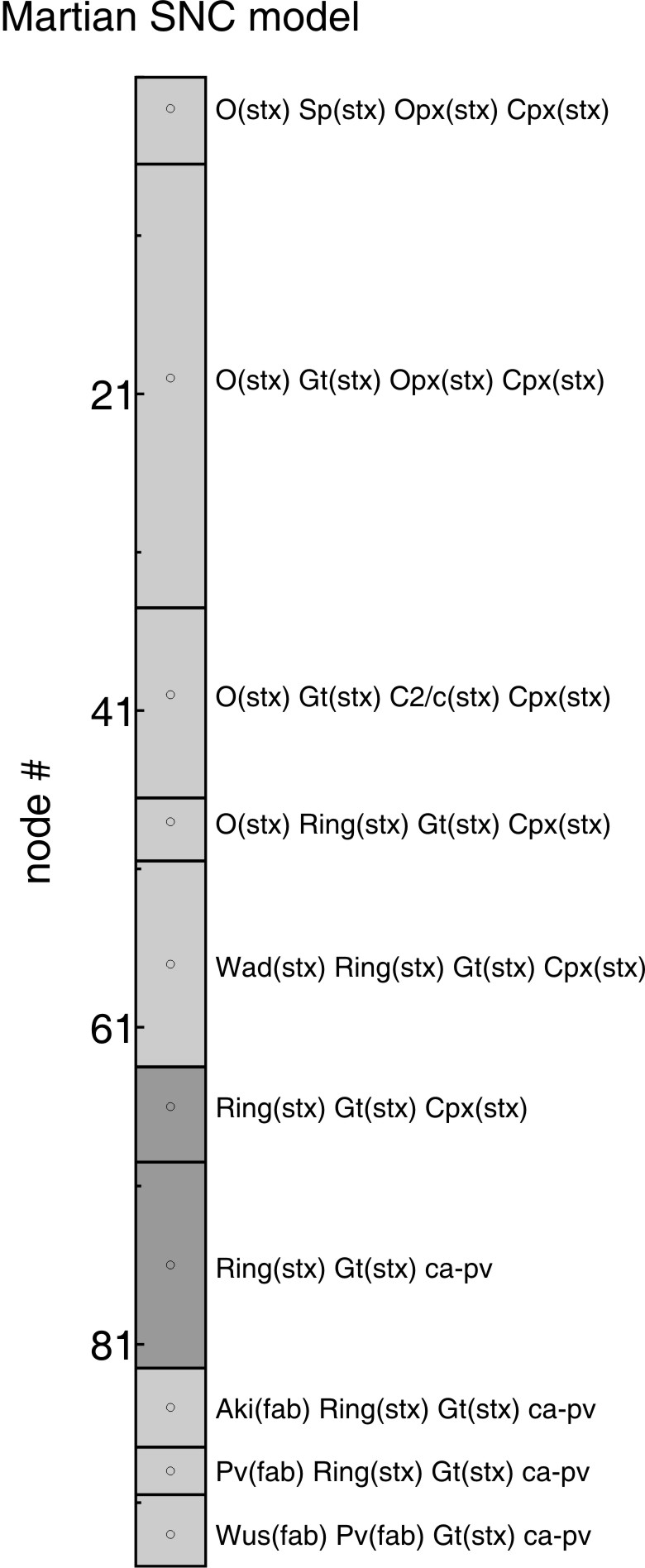
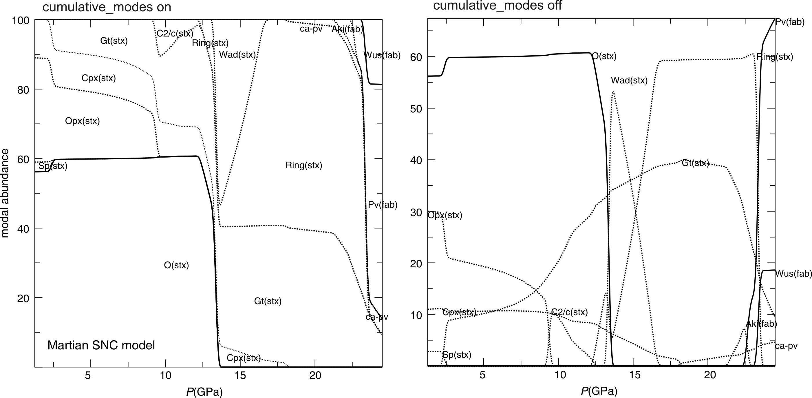
Mantle mineralogy for a Martian model composition and aerotherm. This example Perple_X illustrates calculations for an arbitrary set of physical conditions (i.e., a path) and the use of the "modes of all phases" property choice in WERAMI. The example is outlined in full at perplex_66_example24.
Problem definition file (in24.dat)
Graphical output (pl24.jpg, scpl24.jpg)
Coordinate data file (aerotherm.dat)